Motivation
Chapter 3 established the probabilistic scaffold: given y = X\beta + \varepsilon with \varepsilon \sim \mathcal{N}(0, \sigma^2 I), the OLS estimator \hat\beta = (X^\top X)^{-1} X^\top y is the maximum likelihood estimator, and its sampling covariance is \sigma^2 (X^\top X)^{-1}. That is a clean theoretical result, but it is not yet a tool. An analyst must act — report a coefficient with defensible error bars, decide whether a media channel produced a measurable lift, and explain why adding a correlated predictor sent a previously stable estimate into free fall.
“You fit the model and TV’s coefficient is 2.3. Is that real, how sure are you, and why did the number swing wildly when you added search?”
This chapter converts the estimator into applied methodology. The first stop is optimality: the Gauss–Markov theorem guarantees that OLS achieves the smallest variance among all linear unbiased estimators, which gives the error bars their authority. From the sampling covariance we derive standard errors, t-statistics, and confidence intervals — the machinery that turns 2.3 into “2.3 ± 0.6, p = 0.001” or into “2.3, but the 95% interval spans –1 to 6, so we cannot distinguish signal from noise.”
The second stop is multicollinearity. When TV spend and search spend move together across weeks, X^\top X approaches singularity, \kappa(X) grows large, and \sigma^2 (X^\top X)^{-1} inflates without bound. The coefficient estimates remain unbiased in expectation, but their variance is so large that they are operationally useless — and sensitive to small data perturbations, which is exactly what practitioners observe when adding or removing a correlated channel reshapes all the other coefficients.
The fix introduces a deliberate bias to achieve a large reduction in variance: ridge regression. By penalizing \|\beta\|^2, ridge shrinks the estimates toward zero and stabilizes the inversion. This is the bias–variance tradeoff made concrete. Ridge regression is not merely a numerical patch, however. Interpreted through Bayes’ theorem — which Chapter 3 introduced — the ridge penalty is exactly the log-prior under a Gaussian prior \beta \sim \mathcal{N}(0, \tau^2 I). The penalized least-squares solution is the posterior mode. That equivalence is the bridge to the next chapter on Bayesian inference, where the full posterior replaces point estimates with distributions, and prior specification becomes an explicit modeling choice rather than a regularization hyperparameter (Hastie et al. 2009).
Theory & Proofs
The OLS estimator and its sampling distribution
Proposition (OLS sampling distribution). Under the linear model y = X\beta + \varepsilon with \mathbb{E}[\varepsilon] = 0, \operatorname{Cov}(\varepsilon) = \sigma^2 I, and \varepsilon Gaussian, the OLS estimator \hat\beta = (X^\top X)^{-1} X^\top y is unbiased, has covariance \sigma^2 (X^\top X)^{-1}, and is itself Gaussian:
\hat\beta \sim \mathcal{N}\big(\beta,\ \sigma^2 (X^\top X)^{-1}\big).
Proof. Recall that \hat\beta = (X^\top X)^{-1} X^\top y. To understand its behavior as a random quantity, substitute the data-generating model y = X\beta + \varepsilon directly into this formula. This yields the single most useful decomposition in the chapter:
\hat\beta = (X^\top X)^{-1} X^\top (X\beta + \varepsilon) = \beta + (X^\top X)^{-1} X^\top \varepsilon .
The estimator equals the truth \beta plus a linear image of the noise. Everything that follows reads off this line.
Unbiasedness. Take expectations and use linearity together with the assumption \mathbb{E}[\varepsilon] = 0:
\mathbb{E}[\hat\beta] = \beta + (X^\top X)^{-1} X^\top \mathbb{E}[\varepsilon] = \beta .
So OLS is correct on average: across repeated samples it neither systematically overshoots nor undershoots the true coefficients.
Covariance. The deviation \hat\beta - \beta = (X^\top X)^{-1} X^\top \varepsilon is precisely a linear map A\varepsilon of the noise, with A = (X^\top X)^{-1} X^\top. Applying the transformation identity from Chapter 3, \operatorname{Cov}(Aw) = A \operatorname{Cov}(w) A^\top, with \operatorname{Cov}(\varepsilon) = \sigma^2 I:
\operatorname{Cov}(\hat\beta) = (X^\top X)^{-1} X^\top (\sigma^2 I) X (X^\top X)^{-1} = \sigma^2 (X^\top X)^{-1},
where the collapse uses X^\top X (X^\top X)^{-1} = I and the symmetry of (X^\top X)^{-1}.
Distributional form. Finally, \hat\beta is an affine function of \varepsilon, and an affine function of a Gaussian vector is Gaussian. Combining the mean and covariance just computed:
\hat\beta \sim \mathcal{N}\big(\beta,\ \sigma^2 (X^\top X)^{-1}\big).
\blacksquare
This finite-sample sampling distribution — exact, not asymptotic — is the foundation on which every standard error, t-statistic, and confidence interval in this chapter rests.
Gauss–Markov: OLS is BLUE
The previous result assumed normality. Remarkably, the optimality of OLS does not.
Theorem (Gauss–Markov). Assume only \mathbb{E}[\varepsilon] = 0 and \operatorname{Cov}(\varepsilon) = \sigma^2 I (no normality required). Among all linear unbiased estimators \tilde\beta = Cy, the OLS estimator \hat\beta has the smallest covariance: \operatorname{Cov}(\tilde\beta) - \operatorname{Cov}(\hat\beta) \succeq 0.
Proof. Unbiasedness constrains the estimator. Consider any linear estimator, i.e. \tilde\beta = Cy for some fixed matrix C \in \mathbb{R}^{p \times n} not depending on y. For it to be unbiased for every possible \beta we need
\mathbb{E}[Cy] = \mathbb{E}[C(X\beta + \varepsilon)] = CX\beta = \beta \quad \text{for all } \beta,
which forces the constraint CX = I.
Decompose around the OLS operator. Write
C = (X^\top X)^{-1} X^\top + D,
which simply defines D as the difference. Substituting into CX = I and using (X^\top X)^{-1} X^\top X = I gives I + DX = I, hence the orthogonality condition DX = 0.
Compare covariances. Since \operatorname{Cov}(y) = \sigma^2 I, the transformation identity gives \operatorname{Cov}(\tilde\beta) = \sigma^2 C C^\top. Expanding C C^\top:
\begin{aligned}
\operatorname{Cov}(\tilde\beta) &= \sigma^2 C C^\top \\
&= \sigma^2 \big[(X^\top X)^{-1} X^\top + D\big]\big[X (X^\top X)^{-1} + D^\top\big] \\
&= \sigma^2 \big[(X^\top X)^{-1} + (X^\top X)^{-1} X^\top D^\top + D X (X^\top X)^{-1} + D D^\top\big].
\end{aligned}
The two cross terms vanish: DX = 0 implies X^\top D^\top = (DX)^\top = 0, killing both. What remains is
\operatorname{Cov}(\tilde\beta) = \sigma^2 \big[(X^\top X)^{-1} + D D^\top\big].
Since \operatorname{Cov}(\hat\beta) = \sigma^2 (X^\top X)^{-1}, subtracting gives
\operatorname{Cov}(\tilde\beta) - \operatorname{Cov}(\hat\beta) = \sigma^2 D D^\top \succeq 0,
because any matrix of the form D D^\top is positive semidefinite. Equality holds iff D D^\top = 0, i.e. D = 0, which means \tilde\beta = \hat\beta.
\blacksquare
Gauss–Markov is why OLS is the default estimator: no linear unbiased competitor can do better. But read the theorem’s scope carefully — it certifies OLS as best among unbiased estimators only. That leaves a door open: by tolerating a little bias we may be able to shrink the variance below the Gauss–Markov floor, the maneuver that rungs 6–7 develop into ridge regression.
Estimating the noise level
Every result so far is written in terms of \sigma^2, the variance of the noise — yet \sigma^2 is never observed. To make the sampling distribution operational we must estimate it from the data. The natural raw material is the residual vector \hat\varepsilon = y - X\hat\beta, the part of y that the fit could not explain, and its squared length, the residual sum of squares \text{RSS} = \lVert \hat\varepsilon \rVert^2.
A first instinct is to estimate \sigma^2 by the average squared residual, \text{RSS}/n. This is biased downward. The fitted values are tuned to this very sample, so the residuals are systematically too small: least squares spent some of the data’s variability fitting the p coefficients. Geometrically, the fitted vector X\hat\beta lives in the p-dimensional column space of X, so the residual is confined to the orthogonal complement of that subspace, which has dimension only n - p. The residual has n - p free directions, not n. Dividing by this degrees of freedom rather than by n exactly corrects the bias:
\hat\sigma^2 = \frac{\text{RSS}}{n - p},
which satisfies \mathbb{E}[\hat\sigma^2] = \sigma^2. Beyond unbiasedness, the residual carries a sharper distributional structure. Under the Gaussian model the scaled \text{RSS} follows a chi-square law on the same n - p degrees of freedom, and — crucially — it is independent of the coefficient estimate:
\frac{\text{RSS}}{\sigma^2} \sim \chi^2_{n-p}, \quad \text{independent of } \hat\beta,
a consequence of the orthogonal decomposition of the Gaussian vector, which we take as given (Hastie et al. 2009; Casella and Berger 2002). That independence, paired with the chi-square form, is precisely what makes the next rung’s t-statistic an exact finite-sample pivot rather than a large-sample approximation.
Standard errors, t-tests, and confidence intervals
We now have all the pieces to attach error bars to a coefficient. From rung 1, reading off the j-th diagonal entry of the sampling covariance, the j-th coefficient satisfies
\hat\beta_j \sim \mathcal{N}\big(\beta_j,\ \sigma^2 [(X^\top X)^{-1}]_{jj}\big).
Its true standard deviation is \sigma\sqrt{[(X^\top X)^{-1}]_{jj}}, but \sigma is unknown. Substituting the estimate \hat\sigma from rung 3 yields the standard error, the reported measure of a coefficient’s precision:
\operatorname{se}(\hat\beta_j) = \hat\sigma\sqrt{[(X^\top X)^{-1}]_{jj}}.
Standardizing \hat\beta_j by its true standard deviation would give an exact standard normal. The catch is that we divide instead by the estimated \operatorname{se}. The resulting ratio is a normal variable divided by the square root of an independent scaled chi-square — and that ratio is, by the very definition of the distribution, a Student-t on n - p degrees of freedom:
\frac{\hat\beta_j - \beta_j}{\operatorname{se}(\hat\beta_j)} \sim t_{n-p}.
This is the central pivot of inference. Inverting it — solving for the set of \beta_j consistent with the observed estimate at level 1 - \alpha — produces the confidence interval
\hat\beta_j \pm t_{n-p,\,1-\alpha/2}\,\operatorname{se}(\hat\beta_j).
The same pivot delivers a hypothesis test. To ask whether a media channel’s effect is distinguishable from noise, set H_0: \beta_j = 0; under the null the statistic \hat\beta_j / \operatorname{se}(\hat\beta_j) follows t_{n-p}, so we reject when its magnitude exceeds the t-quantile t_{n-p,\,1-\alpha/2} — the t-test of a single coefficient. When several coefficients must be judged together — say, all of a channel’s lagged terms at once — the analogous F-test compares the drop in \text{RSS} from including them against the residual variance, referred to an F distribution (Hastie et al. 2009). Returning to the Motivation: the coefficient of 2.3 is no longer a bare number. The confidence interval is the precise, defensible answer to “how sure are you?” — distinguishing “2.3 \pm 0.6” from “2.3, but the interval spans -1 to 6.”
Fitted values, residuals, and goodness of fit
Inference so far has concerned the coefficients; we now turn to the fit itself and the assumptions underwriting it. Collecting the fitted values \hat y = X\hat\beta and substituting the OLS formula exposes the linear operator that produces them:
\hat y = X\hat\beta = X(X^\top X)^{-1} X^\top y = Hy, \qquad H = X(X^\top X)^{-1} X^\top .
The matrix H “puts the hat on y,” and is exactly the orthogonal projection onto the column space of X from Chapter 1. It is symmetric and idempotent: H^\top = H because (X^\top X)^{-1} is symmetric, and
H^2 = X(X^\top X)^{-1} X^\top X(X^\top X)^{-1} X^\top = X(X^\top X)^{-1} X^\top = H,
since the inner X^\top X(X^\top X)^{-1} collapses to I. Projecting twice onto a subspace lands in the same place as projecting once. The residual is then \hat\varepsilon = y - \hat y = (I - H)y, the complementary projection onto the orthogonal complement.
To summarize how much of the response the model explains, compare the residual sum of squares against the total variation around the mean. The coefficient of determination is
R^2 = 1 - \frac{\text{RSS}}{\text{TSS}}, \qquad \text{TSS} = \lVert y - \bar y\rVert^2,
the fraction of the variance in y that the fitted model accounts for; R^2 = 1 is a perfect fit and R^2 = 0 is no better than predicting the mean \bar y.
These quantities are only as trustworthy as the four classical assumptions, each of which buys a specific guarantee. Linearity / zero-mean errors (\mathbb{E}[\varepsilon] = 0) buys unbiasedness of \hat\beta (rung 1). Homoscedasticity and uncorrelated errors (\operatorname{Cov}(\varepsilon) = \sigma^2 I) buy the Gauss–Markov optimality (rung 2) and the simple covariance formula \sigma^2 (X^\top X)^{-1}. Normality (\varepsilon Gaussian) buys exact t and F inference (rung 4); without it those become only large-sample approximations. In practice these are checked with residual plots — residuals versus fitted values, residuals versus each predictor, and a normal QQ-plot of the residuals — where curvature, fanning, or heavy tails flag a violated assumption.
Multicollinearity and the bias–variance tradeoff
The covariance \operatorname{Cov}(\hat\beta) = \sigma^2 (X^\top X)^{-1} is benign only when X^\top X is well-conditioned. Because X^\top X is symmetric PSD (Chapter 1), its inverse has eigenvalues 1/\lambda_i; when some \lambda_i is tiny, the corresponding 1/\lambda_i is enormous and the coefficient variances blow up. A small eigenvalue means the columns of X are nearly linearly dependent — collinear media channels whose spend moves together — equivalently a large condition number \kappa(X) (Chapter 1). The estimates stay unbiased but become so variable as to be useless.
The per-coefficient diagnostic is the variance inflation factor
\text{VIF}_j = \frac{1}{1 - R_j^2},
where R_j^2 is the R^2 from regressing predictor j on all the other predictors. A \text{VIF}_j of, say, 100 means \hat\beta_j’s variance is 100 times what it would be if predictor j were orthogonal to the rest.
Escaping this requires admitting biased estimators, which calls for the right yardstick. For any estimator \hat\theta of a scalar \theta:
Proposition. \operatorname{MSE}(\hat\theta) = \mathbb{E}\big[(\hat\theta - \theta)^2\big] = \operatorname{Var}(\hat\theta) + \big(\mathbb{E}[\hat\theta] - \theta\big)^2 — variance plus bias squared.
Proof. Write \mu = \mathbb{E}[\hat\theta]. Adding and subtracting \mu inside the square and expanding,
\begin{aligned}
\operatorname{MSE}(\hat\theta)
&= \mathbb{E}\big[(\hat\theta - \mu)^2\big] + 2(\mu - \theta)\,\mathbb{E}[\hat\theta - \mu] + (\mu - \theta)^2 && \text{(add and subtract $\mu$)} \\
&= \operatorname{Var}(\hat\theta) + (\mu - \theta)^2 && \text{($\mathbb{E}[\hat\theta - \mu] = 0$),}
\end{aligned}
the variance plus the squared bias. \blacksquare
Gauss–Markov (rung 2) makes OLS the minimum-variance estimator among the unbiased ones, but the proposition shows that a biased estimator with much smaller variance can have lower MSE. Under severe collinearity OLS variance is enormous, so accepting a little bias to buy a large variance reduction is a highly favorable trade — exactly the bargain ridge regression (rung 7) walks through next.
Ridge regression: a penalty that is a prior
Ridge regression replaces OLS with penalized least squares, adding a quadratic penalty on the coefficients:
\hat\beta_{\text{ridge}} = \arg\min_\beta\ \lVert y - X\beta\rVert^2 + \lambda\lVert\beta\rVert^2, \qquad \lambda > 0 .
The closed form follows by setting the gradient to zero. The fit term contributes -2X^\top(y - X\beta) (Chapter 2) and the penalty \lambda\lVert\beta\rVert^2 contributes 2\lambda\beta, so
-2X^\top(y - X\beta) + 2\lambda\beta = 0 \ \Longrightarrow\ (X^\top X + \lambda I)\beta = X^\top y \ \Longrightarrow\ \hat\beta_{\text{ridge}} = (X^\top X + \lambda I)^{-1} X^\top y .
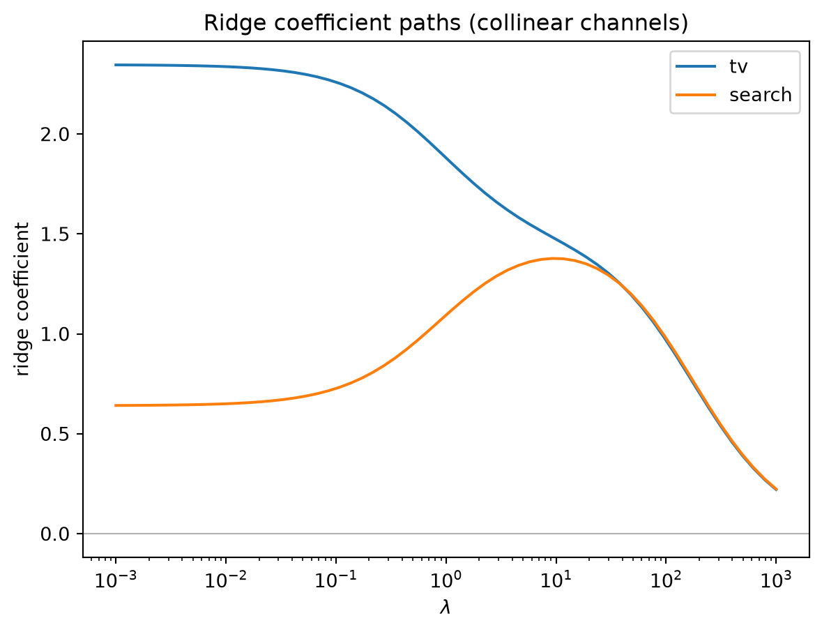
This is precisely the conditioning fix for rung 6. Adding \lambda I shifts every eigenvalue of the symmetric PSD matrix X^\top X (Chapter 1) from \lambda_i to \lambda_i + \lambda. Even when some \lambda_i \approx 0 — severe collinearity, a huge condition number \kappa(X) — the shifted matrix is comfortably invertible and its inverse is well-behaved, so the exploding variances are tamed. The cure has a price: the coefficients are deliberately shrunk toward zero, trading the unbiasedness of OLS for bias. As \lambda grows the estimator’s variance shrinks while that bias grows — the bias–variance trade of rung 6 made into a tunable dial.
Why a squared-error penalty, of all choices? Because it is secretly a Gaussian prior.
Theorem (ridge = Gaussian-prior MAP). Under the model y\sim\mathcal N(X\beta,\sigma^2 I) with prior \beta\sim\mathcal N(0,\tau^2 I), the posterior mode (MAP estimate) of \beta is exactly the ridge estimator with \lambda = \sigma^2/\tau^2.
Proof. By Bayes’ theorem (Chapter 3), p(\beta\mid y)\propto p(y\mid\beta)\,p(\beta). Both factors are Gaussian densities, so taking logs turns each into a negative quadratic:
\log p(\beta\mid y) = -\frac{1}{2\sigma^2}\lVert y - X\beta\rVert^2 \;-\; \frac{1}{2\tau^2}\lVert\beta\rVert^2 \;+\; \text{const},
where the constant collects all terms free of \beta. The MAP estimate maximizes this; multiplying by -2\sigma^2 flips the maximization into a minimization,
\hat\beta_{\text{MAP}} = \arg\min_\beta\ \lVert y - X\beta\rVert^2 + \frac{\sigma^2}{\tau^2}\lVert\beta\rVert^2 ,
which is exactly the ridge objective with \lambda = \sigma^2/\tau^2, whose minimizer we computed above as (X^\top X + \lambda I)^{-1}X^\top y.
\blacksquare
So a penalty is a prior. A tighter prior — small \tau^2, expressing strong belief that coefficients are near zero — yields a larger \lambda and heavier shrinkage, while a vague prior \tau^2\to\infty sends \lambda\to0 and recovers OLS. Changing the penalty changes the prior: an \ell_1 penalty \lambda\lVert\beta\rVert_1 is a Laplace prior, giving lasso and its sparse, variable-selecting solutions, and combining the two penalties gives the elastic-net. The next chapter takes this view to its conclusion: Bayesian inference keeps the entire posterior p(\beta\mid y) rather than just its mode, turning regularization strength from a tuning knob into an explicit modeling choice.
Advanced track — generalized linear models and link functions. The core path does not depend on this; it is the foundation for the optional log-link likelihood discussed in Part V.
Everything above assumes the mean responds linearly to the features and the noise is additive Gaussian, y \sim \mathcal{N}(X\beta,\, \sigma^2 I). Two consequences are baked in: the model can predict negative outcomes, and the noise has constant variance \sigma^2 regardless of the level of X\beta. Neither holds for revenue, which is strictly positive and whose spread typically grows with its level.
A generalized linear model (GLM) keeps the linear predictor \eta = X\beta but inserts a link function g between it and the mean, g(\mathbb{E}[y \mid X]) = X\beta, and pairs it with a response distribution from the exponential family. The choice g = \log — the log link — gives \mathbb{E}[y \mid X] = \exp(X\beta), which is positive for every \beta and turns additive effects on the linear scale into multiplicative effects on the response, so a coefficient reads as a percentage lift rather than a dollar increment. Combined with a lognormal or Gamma response it also lets the variance scale with the mean, repairing the heteroscedasticity the additive Gaussian form ignores.
The MMM in this book deliberately stays with the additive Gaussian likelihood, because additivity is what makes per-channel contributions sum to total predicted sales and keeps each channel’s response curve separable for the budget optimizer of Part IV. The log link is the narrow, principled escape hatch when positivity or variance-scaling genuinely bites — adopted as a likelihood swap, not a redesign of the contribution structure. We return to it in Part V.
Worked Examples
Example: a coefficient with its confidence interval
The theory rungs are most convincing when carried through by hand. Take a deliberately tiny problem — an intercept and a single media channel observed over four weeks, with n = 4 and p = 2:
X = \begin{bmatrix} 1 & 1 \\ 1 & 2 \\ 1 & 3 \\ 1 & 4 \end{bmatrix}, \qquad y = \begin{bmatrix} 2 \\ 2 \\ 4 \\ 5 \end{bmatrix}.
The normal-equation ingredients. Form the cross-product matrix and the cross-product vector that the OLS formula requires:
X^\top X = \begin{bmatrix} 4 & 10 \\ 10 & 30 \end{bmatrix}, \qquad X^\top y = \begin{bmatrix} 13 \\ 38 \end{bmatrix}.
The determinant of X^\top X is 4\cdot 30 - 10\cdot 10 = 20, so the inverse follows from the 2\times 2 rule (swap the diagonal, negate the off-diagonal, divide by the determinant):
(X^\top X)^{-1} = \frac{1}{20}\begin{bmatrix} 30 & -10 \\ -10 & 4 \end{bmatrix} = \begin{bmatrix} 1.5 & -0.5 \\ -0.5 & 0.2 \end{bmatrix}.
The coefficients. Apply \hat\beta = (X^\top X)^{-1} X^\top y:
\hat\beta = \begin{bmatrix} 1.5 & -0.5 \\ -0.5 & 0.2 \end{bmatrix}\begin{bmatrix} 13 \\ 38 \end{bmatrix} = \begin{bmatrix} 1.5\cdot 13 - 0.5\cdot 38 \\ -0.5\cdot 13 + 0.2\cdot 38 \end{bmatrix} = \begin{bmatrix} 0.5 \\ 1.1 \end{bmatrix}.
The intercept is \hat\beta_0 = 0.5 and the channel’s slope is \hat\beta_1 = 1.1: each additional unit of spend is associated with a 1.1-unit lift in the response.
Residuals and the noise estimate. The fitted values are \hat y = X\hat\beta, namely 0.5 + 1.1\,x evaluated at x = 1,2,3,4:
\hat y = \begin{bmatrix} 1.6 \\ 2.7 \\ 3.8 \\ 4.9 \end{bmatrix}, \qquad \hat\varepsilon = y - \hat y = \begin{bmatrix} 0.4 \\ -0.7 \\ 0.2 \\ 0.1 \end{bmatrix}.
Summing the squared residuals gives the residual sum of squares,
\text{RSS} = 0.4^2 + (-0.7)^2 + 0.2^2 + 0.1^2 = 0.16 + 0.49 + 0.04 + 0.01 = 0.70,
and dividing by the n - p = 4 - 2 = 2 residual degrees of freedom estimates the noise variance:
\hat\sigma^2 = \frac{\text{RSS}}{n - p} = \frac{0.70}{2} = 0.35, \qquad \hat\sigma = \sqrt{0.35} \approx 0.5916 .
Standard error and confidence interval. The slope is the coefficient \hat\beta_1, so (indexing the matrix to match, with the intercept as entry 0) its standard error reads off the [(X^\top X)^{-1}]_{11} = 0.2 entry:
\operatorname{se}(\hat\beta_1) = \hat\sigma\sqrt{[(X^\top X)^{-1}]_{11}} = \sqrt{0.35}\,\sqrt{0.2} = \sqrt{0.07} \approx 0.2646 .
With n - p = 2 degrees of freedom the relevant Student-t quantile is t_{2,\,0.975} \approx 4.303, far larger than the familiar 1.96 because two degrees of freedom is a very thin sample. The 95% confidence interval for the slope is therefore
\hat\beta_1 \pm t_{2,\,0.975}\,\operatorname{se}(\hat\beta_1) = 1.1 \pm 4.303 \times 0.2646 = 1.1 \pm 1.138 = [-0.038,\ 2.238].
The point estimate 1.1 looks like a clear positive effect, yet the interval only just dips below zero: equivalently, the test statistic \hat\beta_1/\operatorname{se}(\hat\beta_1) = 1.1/0.2646 \approx 4.158 falls a hair short of the critical 4.303, so at the 5% level we cannot reject \beta_1 = 0. This is exactly the Motivation’s cautionary tale made arithmetic — a healthy-looking coefficient whose error bars, on four weeks of data, refuse to certify it as signal.
Example: collinearity and the ridge remedy
Now the second failure mode of the Motivation: two media channels whose spend moves together. Over six weeks, let channel 1 take the values x_1 = (1,2,3,4,5,6) and let channel 2 be a near-duplicate, x_2 = (1.1,\,1.9,\,3.1,\,3.9,\,5.1,\,5.9) — the same upward trend jittered by \pm 0.1. With an intercept the design and response are
X = \begin{bmatrix} 1 & 1 & 1.1 \\ 1 & 2 & 1.9 \\ 1 & 3 & 3.1 \\ 1 & 4 & 3.9 \\ 1 & 5 & 5.1 \\ 1 & 6 & 5.9 \end{bmatrix}, \qquad y = \begin{bmatrix} 3.1 \\ 4.0 \\ 6.2 \\ 7.1 \\ 9.3 \\ 9.9 \end{bmatrix}.
OLS on the collinear design. Solving the normal equations (all figures rounded to three decimals) gives
\hat\beta_{\text{OLS}} = \begin{bmatrix} 1.306 \\ -2.050 \\ 3.563 \end{bmatrix}, \qquad \operatorname{se} = \begin{bmatrix} 0.108 \\ 0.470 \\ 0.477 \end{bmatrix}.
The result is nonsense as channel attribution: although both channels carry the same rising signal, OLS assigns one a large negative coefficient (-2.050) and the other a large positive one (3.563). The estimator has split a modest joint effect into two enormous, nearly cancelling pieces — their sum, -2.050 + 3.563 = 1.513, is the only stable quantity. The diagnostics confirm the pathology: the condition number is \kappa(X) \approx 81.8, and the variance inflation factor for each channel is
\text{VIF} = \frac{1}{1 - R_j^2} = \frac{1}{1 - 0.99677} \approx 309 ,
so each slope’s variance is roughly 309 times — and its standard error about \sqrt{309} \approx 17.6 times — what an orthogonal design would deliver. The two channels are individually unidentifiable; the data simply cannot say how to apportion credit between them.
Ridge stabilizes the split. Apply the ridge estimator \hat\beta_{\text{ridge}} = (X^\top X + \lambda I)^{-1} X^\top y with a modest penalty \lambda = 1:
\hat\beta_{\text{ridge}} = \begin{bmatrix} 0.861 \\ 0.706 \\ 0.892 \end{bmatrix}.
The shift of every eigenvalue of X^\top X by \lambda = 1 (rung 7) cures the near-singular inversion. Both channel coefficients are now positive and close together — 0.706 and 0.892, a spread of 0.186 rather than the OLS spread of |3.563 - (-2.050)| = 5.613 — and each sits at a sensible value reflecting that the two near-identical channels should receive near-identical credit. The wild sign flip is gone. The price, as the theory insists, is bias: the coefficients are shrunk toward zero (and their sum, 1.598, no longer matches the OLS sum exactly), but in exchange for a collinear design that OLS rendered uninterpretable, ridge returns coefficients an analyst can actually report.
Exercises
C – Conceptual / Reading Comprehension
C1. Suppose you fit the media-mix model and report a 95% confidence interval [1.514,\,2.048] for the TV coefficient \beta_{\text{TV}}. State carefully what this interval claims and what it does not claim. In particular, address the common misreading that “there is a 95% probability that the true \beta_{\text{TV}} lies in [1.514,\,2.048].” Why is that statement wrong under the frequentist sampling-distribution \hat\beta\sim\mathcal N(\beta,\sigma^2(X^\top X)^{-1}), and what is the correct probabilistic object the 95\% actually refers to?
C2. Two media channels (say TV and a near-duplicate “search” spend that tracks it closely) are strongly collinear, yet the model’s overall fit R^2 is excellent. Explain why the individual coefficient standard errors can nonetheless be enormous. Tie your explanation explicitly to the matrix (X^\top X)^{-1}: which quantity in \operatorname{se}(\hat\beta_j)=\hat\sigma\sqrt{[(X^\top X)^{-1}]_{jj}} blows up, what near-singularity of X^\top X does to its inverse, and why a great joint fit is fully compatible with terrible individual coefficient precision.
C3. Ridge regression replaces \hat\beta=(X^\top X)^{-1}X^\top y with (X^\top X+\lambda I)^{-1}X^\top y, which is a biased estimator of \beta. What does this deliberate bias buy in return, and how should one think about the resulting bias–variance tradeoff as \lambda grows? Then explain in what precise sense choosing the penalty \lambda is the same thing as choosing a Gaussian prior \beta\sim\mathcal N(0,\tau^2 I), including the identification \lambda=\sigma^2/\tau^2 and what \lambda\to 0 and \lambda\to\infty correspond to in prior terms.
B – By Hand
B1. Let
X=\begin{bmatrix}1&1\\1&2\\1&3\\1&4\end{bmatrix},
\qquad
y=\begin{bmatrix}2\\2\\4\\5\end{bmatrix}.
Compute the OLS estimate \hat\beta=(X^\top X)^{-1}X^\top y (intercept and slope). Then compute the residual sum of squares \text{RSS}=\lVert y-X\hat\beta\rVert^2, the noise estimate \hat\sigma^2=\text{RSS}/(n-p) with n=4 and p=2, and the standard error of the slope \operatorname{se}(\hat\beta_1)=\hat\sigma\sqrt{[(X^\top X)^{-1}]_{11}} (index the slope as j=1). Show your intermediate matrices.
B2. Two predictors enter a regression and have sample correlation r=0.95. Using the two-predictor identity R_j^2=r^2, compute the variance inflation factor \text{VIF}_j=1/(1-R_j^2) for each predictor. By what factor does the collinearity inflate the variance of each coefficient relative to an orthogonal design, and what does that imply for the standard errors (which scale as \sqrt{\text{VIF}_j})?
B3. Given
X^\top X=\begin{bmatrix}4&2\\2&4\end{bmatrix},
\qquad
X^\top y=\begin{bmatrix}6\\4\end{bmatrix},
compute the ridge estimate \hat\beta_{\text{ridge}}=(X^\top X+\lambda I)^{-1}X^\top y at \lambda=2. Form X^\top X+\lambda I, invert it explicitly, and report \hat\beta_{\text{ridge}}. For comparison, also compute the OLS estimate (\lambda=0) and comment on how the penalty has shrunk the coefficients.
P – Prove It
P1. Assume the linear model y=X\beta+\varepsilon with fixed (non-random) design X of full column rank and \mathbb{E}[\varepsilon]=0. Prove that the OLS estimator \hat\beta=(X^\top X)^{-1}X^\top y is unbiased, i.e. \mathbb{E}[\hat\beta]=\beta. State clearly where you use linearity of expectation and the assumption \mathbb{E}[\varepsilon]=0.
P2. Adopt the Gauss–Markov assumptions: \mathbb{E}[\varepsilon]=0 and \operatorname{Cov}(\varepsilon)=\sigma^2 I, with X fixed and full column rank. Consider any linear estimator \tilde\beta=Cy that is unbiased for every \beta. Prove the Gauss–Markov theorem: the OLS estimator \hat\beta=(X^\top X)^{-1}X^\top y has the smallest covariance among all such \tilde\beta, in the sense that \operatorname{Cov}(\tilde\beta)-\operatorname{Cov}(\hat\beta) is positive semidefinite. (Hint: write C=(X^\top X)^{-1}X^\top+D, show unbiasedness forces DX=0, and expand the covariance.)
P3. Suppose y\mid\beta\sim\mathcal N(X\beta,\sigma^2 I) with the Gaussian prior \beta\sim\mathcal N(0,\tau^2 I). Prove that the maximum a posteriori (MAP) estimate of \beta — the maximizer of the posterior p(\beta\mid y) — equals the ridge estimator (X^\top X+\lambda I)^{-1}X^\top y, and show that the penalty is identified as \lambda=\sigma^2/\tau^2. (Hint: maximize the log-posterior, i.e. minimize \tfrac{1}{\sigma^2}\lVert y-X\beta\rVert^2+\tfrac{1}{\tau^2}\lVert\beta\rVert^2, by setting the gradient to zero.)
A – Applied / Code
A1. Sampling variability of OLS. Build a fixed two-channel design matrix X (an intercept plus two media channels) whose two channel columns have a target correlation \rho, and pick a true coefficient vector \beta_{\text{true}}. For each \rho\in\{0,\,0.9,\,0.99\}, hold X fixed and draw many response vectors y=X\beta_{\text{true}}+\varepsilon with \varepsilon\sim\mathcal N(0,\sigma^2 I); refit OLS on each draw and collect the estimated coefficient \hat\beta_{\text{search}} for the second channel across the draws. Plot (e.g. histograms or overlaid densities) showing the empirical spread of \hat\beta_{\text{search}} widening as \rho increases. For each \rho, overlay the theoretical standard deviation \sigma\sqrt{[(X^\top X)^{-1}]_{jj}} (where j indexes the search coefficient) and confirm that the empirical standard deviation of your \hat\beta_{\text{search}} samples matches it.
A2. Bias–variance experiment, OLS vs. ridge. Fix a strongly collinear design X and a true coefficient vector \beta_{\text{true}}. Simulate many datasets y=X\beta_{\text{true}}+\varepsilon; on each, compute the OLS estimate and the ridge estimate (X^\top X+\lambda I)^{-1}X^\top y over a grid of \lambda values. For each estimator, average the squared recovery error \lVert\hat\beta-\beta_{\text{true}}\rVert^2 across datasets to estimate its mean-squared error. Plot MSE versus \lambda (with the OLS MSE shown as the \lambda=0 reference), and identify a value \lambda>0 at which ridge achieves lower MSE than OLS. Comment on how the curve illustrates the bias–variance tradeoff.