Motivation
Chapter 18 (Budget Optimization) ran the Part IV optimizer against the Chapter 16 posterior and returned a result that looked like a decision: allocate (7.2, 1.8) across two channels, shadow price \lambda^\star \approx 0.3727, total response 6.7082. Run against the full posterior instead of its mean, the same optimizer revealed that the confident allocation sits inside a credible region spanning more than four budget units out of nine — every point in that band reproducing the historical sales series equally well while implying materially different channel investments. Chapter 16 (Building and Fitting an MMM) named the geometry behind this width the identifiability ridge: directions in parameter space that observational spend data leave nearly flat. Chapter 18 quantified its cost as the expected value of perfect information and left the wound open. Chapter 19 names the reason the wound exists.
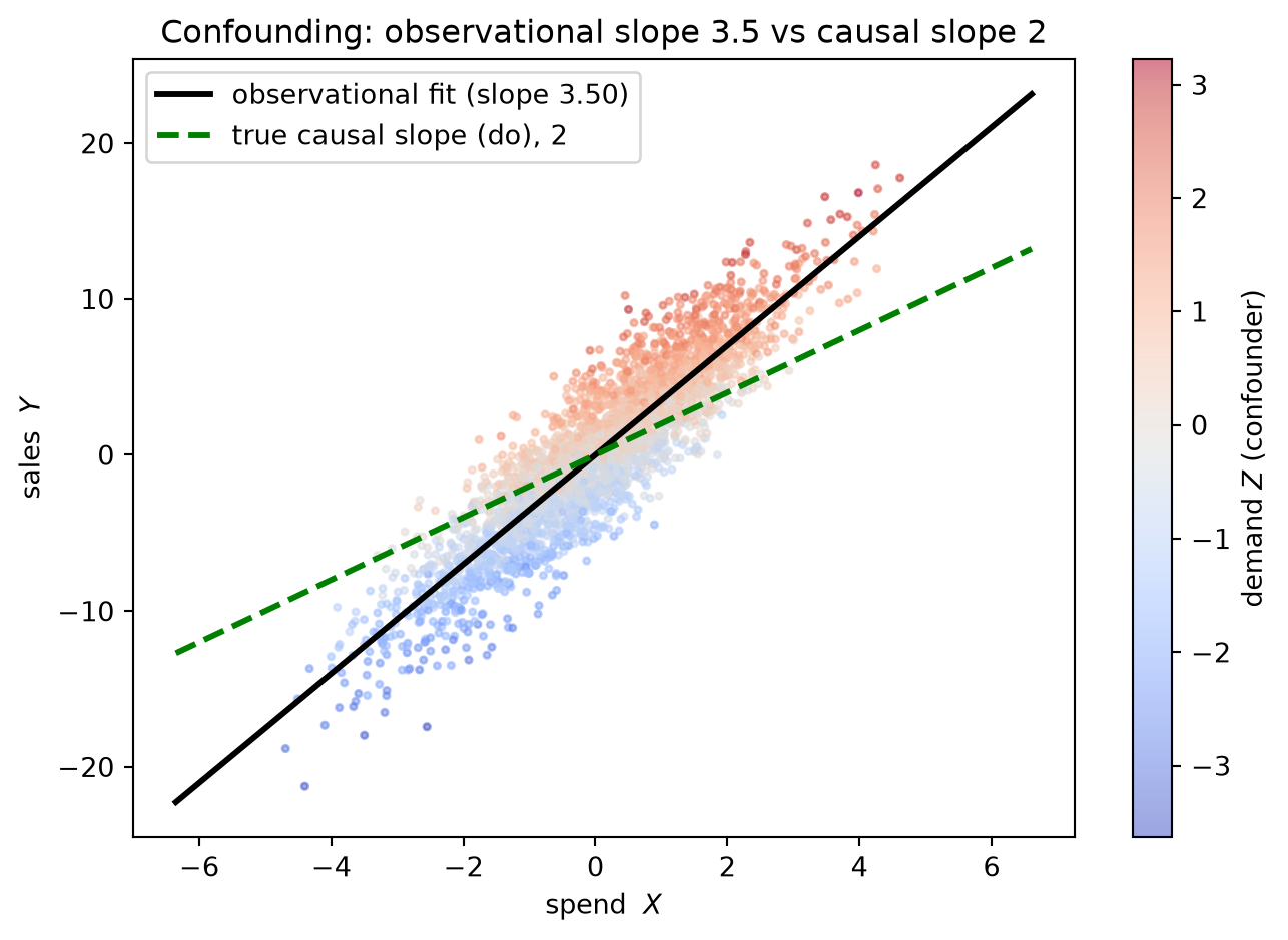
The reason is endogeneity of spend. A marketing manager planning for a high-demand quarter — a retail season, a pre-announced product launch, an external demand surge she can read from forward bookings — does not hold spend constant; she increases it, because the expected return on advertising is higher when baseline demand is already elevated. The decision is rational. Its consequence for regression is structural: spend is positively correlated with a demand driver that also moves sales through a channel the model does not contain. A regression of sales on spend then picks up both effects in the same coefficient — part genuine causal lift from the advertising, part elevated baseline demand that would have been there whether the ads ran or not. The fitted slope is an average over both, and the bias runs in the direction that makes advertising look better than it is. Chapter 4 (Linear Regression) planted exactly this teaser when it noted that the OLS slope is unbiased only when regressors are uncorrelated with the residual; in an observational MMM, that assumption fails structurally, not accidentally. No amount of additional observational data removes the bias. It only pins the biased number with greater precision.
The chapter’s driving question follows directly: a fitted coefficient is causal only under conditions we must name. This chapter names them. Naming them requires a language the time-series machinery of Chapters 15 and 16 did not provide — a formal vocabulary for distinguishing what the data generate from what an intervention would generate. The chapter develops two complementary frameworks to supply that vocabulary.
The first is potential outcomes: for each observation and each spend level x, there is a sales outcome Y_i(x) the system would have produced had spend been set to x, regardless of what spend actually was. The causal effect of moving spend from x to x' is Y_i(x') - Y_i(x), a comparison of two counterfactual worlds the data can reveal at most one of.
The second framework is the do-operator of causal graphs: \mathrm{do}(X = x) represents an intervention that sets spend by external force, severing the correlation with the demand driver that created the confound. The difference between P(Y \mid X = x) — the conditional distribution of sales when spend is observed to equal x — and P(Y \mid \mathrm{do}(X = x)) — the distribution when spend is set to x — is precisely the gap between a correlation and a causal effect.
The chapter leads with potential outcomes, which connect directly to the regression framework of Chapter 4, and then bridges to causal graphs and directed acyclic graphs (DAGs), which supply the graphical language for reading off what must be conditioned on to recover a causal estimate and what cannot be.
The chapter’s payoff runs through a single worked example that makes the cost of confounding arithmetic. A synthetic MMM with one spend channel and one unobserved demand driver is constructed so the true causal effect of spend on sales is known. The demand driver elevates both spend — because the manager responds to it — and baseline sales — because customers respond to it — creating a positive confound. The naive response slope, fit on the observational time series, overstates the true causal effect by seventy-five percent. Controlling for the demand driver recovers the truth. The wound this example makes concrete is that in a realistic MMM the demand driver is almost never observed: it is the very correlated baseline that motivated the identifiability ridge of Chapter 16. When the confounder lives in the error term, the observational regression is fundamentally limited, which is why Part VI must turn to direct experimentation. Chapter 20 (Quasi-Experimental Designs) shows how geo-holdouts and matched-market tests generate spend variation that is, by design, uncorrelated with the demand driver — producing identification the observational series cannot supply. Chapter 21 (Advanced Calibration) folds those identified estimates back into the posterior as likelihood factors, compressing the ridge in the direction the optimizer requires and shrinking the EVPI gap that Chapter 18 could only name.
Theory & Proofs
The first three rungs build the chapter’s causal vocabulary and prove its central bias result. Rung 1 introduces potential outcomes and names the fundamental problem of causal inference — the observability constraint that makes the response curve an inherently counterfactual object. Chapter 16 (Building & Fitting an MMM) estimated the MMM parameters from observational spend data; the question this chapter answers is whether the fitted slopes equal the causal response the Part IV optimizer requires. Rung 2 defines the conditions under which an observational regression recovers a causal estimate, derives the adjustment formula, and names the estimand Chapter 18 (Budget Optimization) consumed. Rung 3 proves the chapter’s keystone result: the omitted-variable bias theorem, showing that the naive MMM slope is a biased estimator of the causal response whenever spend is endogenous and the confounder moves sales — and that the bias does not vanish with more data.
Rung 1 — The causal question in MMM (potential outcomes)
The potential-outcomes framework. For each time period i and each possible spend level x, define Y_i(x) as the sales period i would have produced had spend been set to x — regardless of the spend X_i that was actually observed. The function x \mapsto Y_i(x) is period i’s potential-outcome schedule: a complete description of how that period’s sales respond to every counterfactual spend level. Its population expectation is the dose–response curve,
\mu(x) = \mathbb{E}[Y_i(x)],
and it is exactly the object Chapter 18 (Budget Optimization) operated on: the equal-marginal allocation, the shadow price \lambda^\star, and the envelope-theorem scenario analysis all act on \mu and its slope d\mu/dx. A higher slope means a higher marginal return on spend; the Chapter 18 optimizer directs more budget toward the steeper channel. Whether the fitted MMM response curve equals \mu — and therefore whether the Chapter 18 allocation is trustworthy — is the question the present chapter is designed to answer.
The fundamental problem of causal inference. At every period i, only one potential outcome is ever observed — the one corresponding to the spend that actually occurred:
Y_i^{\text{obs}} = Y_i(X_i).
For any x \neq X_i the value Y_i(x) is a counterfactual — it is never directly available in the data. This observability constraint is the fundamental problem of causal inference: causal effects are comparisons across potential outcomes, but data supply only one potential outcome per period. The fitted MMM regression of Y_i^{\text{obs}} on X_i returns a slope; whether that slope equals d\mu/dx depends entirely on why X_i took the values it did. Chapter 4 (Linear Regression) established that the OLS slope is unbiased only when the regressor is uncorrelated with the residual; in an observational MMM, spend is an endogenous management decision, not a randomized treatment. A manager who increases spend in high-demand periods introduces a structural correlation between the regressor and the error, and the OLS slope absorbs both the causal advertising effect and the elevated baseline demand into a single coefficient. Rung 2 formalizes when that absorption is harmless, and Rung 3 quantifies when it is not.
Rung 2 — Ignorability and the observational/interventional gap
Unconfoundedness (ignorability). Let Z_i denote the vector of demand-state covariates for period i. The spend assignment is unconfounded (or ignorable) given Z if
Y_i(x) \perp X_i \;\Big|\; Z_i \quad \text{for all } x.
Read: among periods sharing the same demand state Z_i = z, the level of spend X_i is “as good as randomly assigned” — potential outcomes carry no residual dependence on which spend level was chosen once Z is held fixed. Intuitively, Z blocks every back-door pathway by which a manager’s anticipation of high demand could simultaneously inflate spend and baseline sales.
Positivity (overlap). The companion condition requires that every spend level has positive probability at each demand state:
P(X_i = x \mid Z_i = z) > 0 \quad \text{for all } x \text{ in the support of } X \text{ and all } z \text{ in the support of } Z.
Without positivity, no data at covariate value z can inform the conditional mean \mathbb{E}[Y \mid X = x, Z = z] at untested spend levels, and the adjustment formula below is undefined at those cells.
Recovery of the dose–response by adjustment. Under ignorability and positivity,
\mu(x) = \mathbb{E}_Z\bigl[\,\mathbb{E}[Y \mid X = x,\, Z]\,\bigr].
Derivation. Condition on Z and apply ignorability. Since Y = Y(X), conditioning on X = x pins the observed outcome to Y(x):
\begin{aligned}
\mathbb{E}[Y \mid X = x,\, Z]
&= \mathbb{E}[Y(x) \mid X = x,\, Z] \\[4pt]
&= \mathbb{E}[Y(x) \mid Z],
\end{aligned}
where the first equality uses Y = Y(X) evaluated at X = x, and the second uses ignorability (Y_i(x) \perp X_i \mid Z_i), which allows dropping the conditioning on X = x. Averaging over Z by the law of iterated expectations:
\mathbb{E}_Z\bigl[\,\mathbb{E}[Y \mid X = x,\, Z]\,\bigr]
= \mathbb{E}_Z\bigl[\,\mathbb{E}[Y(x) \mid Z]\,\bigr]
= \mathbb{E}[Y(x)]
= \mu(x).
The observational/interventional gap. The adjustment formula marginalizes over Z at each fixed spend level x. The naive regression conditional \mathbb{E}[Y \mid X = x] skips that marginalization: it is average sales across periods where spend happened to equal x, with demand states appearing in whatever proportions they co-occur with spend level x in the data. When spend and demand are positively correlated — as they are when managers rationally increase spend in high-demand periods — periods with X_i = x over-represent high-Z states, and \mathbb{E}[Y \mid X = x] exceeds the causal \mu(x). The discrepancy is confounding bias, and it is not a sampling artifact: it reflects a structural mismatch between the observational distribution and the interventional distribution the optimizer requires.
The estimand. The quantity Chapter 18 (Budget Optimization) needs is the causal response slope,
\frac{d\mu}{dx}
= \frac{d}{dx}\,\mathbb{E}_Z\bigl[\,\mathbb{E}[Y \mid X = x,\, Z]\,\bigr].
This is the marginal return on spend in the causal sense: the expected gain in sales from increasing spend by one unit, where spend is set by intervention rather than observed. Rung 3 proves, in a linear structural model, exactly how far the OLS slope deviates from this target when the ignorability condition fails.
Rung 3 — Proof P1 (KEYSTONE): the omitted-variable / confounding bias theorem
Structural setup. The data-generating process is a two-equation structural model. The outcome equation encodes the true causal response:
Y = \beta X + \gamma Z + \varepsilon,
where \varepsilon is mean-zero and independent of (X, Z). The coefficient \beta is the causal response slope — the parameter the MMM must recover for the Chapter 18 (Budget Optimization) optimizer to be trustworthy. The covariate Z is a demand driver that shifts baseline sales with coefficient \gamma. The spend equation captures endogenous budgeting:
X = \delta Z + \nu,
where \nu is mean-zero and independent of Z (and of \varepsilon). When \delta \neq 0, spend tracks the demand state, introducing the structural correlation \operatorname{cov}(X, Z) = \delta\,\operatorname{var}(Z) that a regression of Y on X alone cannot separate from the causal effect of spend.
Theorem. The probability limit of the naive least-squares regression of Y on X alone is
\operatorname{plim}\,\hat\beta_{\mathrm{naive}}
= \frac{\operatorname{cov}(X,\,Y)}{\operatorname{var}(X)}
= \beta + \gamma\,\frac{\operatorname{cov}(X,\,Z)}{\operatorname{var}(X)}.
Proof. By the standard probability-limit form of the OLS slope in a simple regression, \operatorname{plim}\,\hat\beta_{\mathrm{naive}} = \operatorname{cov}(X,Y)/\operatorname{var}(X). Expand the numerator using Y = \beta X + \gamma Z + \varepsilon:
\begin{aligned}
\operatorname{cov}(X,\,Y)
&= \operatorname{cov}(X,\;\beta X + \gamma Z + \varepsilon) \\[4pt]
&= \beta\,\operatorname{var}(X)
+ \gamma\,\operatorname{cov}(X,\,Z)
+ \operatorname{cov}(X,\,\varepsilon).
\end{aligned}
Because \varepsilon is independent of (X, Z) by assumption, \operatorname{cov}(X, \varepsilon) = 0. Dividing by \operatorname{var}(X):
\operatorname{plim}\,\hat\beta_{\mathrm{naive}}
= \frac{\beta\,\operatorname{var}(X) + \gamma\,\operatorname{cov}(X,\,Z)}{\operatorname{var}(X)}
= \beta + \gamma\,\frac{\operatorname{cov}(X,\,Z)}{\operatorname{var}(X)}. \quad\blacksquare
Reading the bias. The second term is the omitted-variable bias (OVB):
\text{Bias} = \gamma\,\frac{\operatorname{cov}(X,\,Z)}{\operatorname{var}(X)}.
It is zero if and only if \operatorname{cov}(X,Z) = 0 (spend exogenous, \delta = 0) or \gamma = 0 (Z does not affect sales). In the MMM setting both conditions fail structurally: managers rationally track demand (\delta \neq 0) and demand genuinely moves sales (\gamma \neq 0). Crucially, the bias does not shrink with sample size — it is a property of the joint distribution of (X, Z), not of sampling noise. Adding more data pins the biased number \operatorname{plim}\,\hat\beta_{\mathrm{naive}} with greater precision; it does not move it toward the true \beta. Chapter 4 (Linear Regression) noted that OLS is unbiased under \operatorname{cov}(X, \varepsilon) = 0; endogeneity violates that condition, and the theorem above makes the violation’s cost exact. This is the rigorous statement of Chapter 18’s wound: not a finite-sample imprecision, but a structural feature of endogenous spend.
Analytic anchor. Set \beta = 2, \gamma = 3, \delta = 1, \operatorname{var}(Z) = 1, \operatorname{var}(\nu) = 1. From the spend equation X = Z + \nu:
\operatorname{cov}(X,\,Z) = \delta\,\operatorname{var}(Z) = 1, \qquad
\operatorname{var}(X) = \delta^2\,\operatorname{var}(Z) + \operatorname{var}(\nu) = 1 + 1 = 2.
Therefore
\text{Bias} = \gamma\,\frac{\operatorname{cov}(X,\,Z)}{\operatorname{var}(X)} = 3 \cdot \frac{1}{2} = 1.5, \qquad
\operatorname{plim}\,\hat\beta_{\mathrm{naive}} = 2 + 1.5 = 3.5.
The naive regression returns 3.5 for a true causal slope of \beta = 2 — a 75\% overstatement. These are the running numbers the chapter uses throughout: the Worked Examples and Code Tie-in recover them by simulation and direct regression, and the companion rungs 4–6 show how the do-operator and DAG back-door criterion trace the same bias through the causal graph.
Rung 4 — Structural causal models, DAGs, and the do-operator
Structural causal model. The two structural equations of Rung 3 describe not merely a statistical model but a generative mechanism — a causal recipe by which nature produces data. Reading them as an SCM: Z is set by exogenous forces outside the model; X is then determined by the manager’s response to Z plus idiosyncratic noise \nu; finally Y is produced as a function of X, Z, and independent noise \varepsilon. The independence of the noise terms, together with the causal ordering, defines the structural causal model (SCM):
\begin{aligned}
X &= \delta Z + \nu, \\
Y &= \beta X + \gamma Z + \varepsilon,
\end{aligned}
with \nu \perp Z, \varepsilon \perp (X, Z), and all noise terms mutually independent. The equations are not symmetric: Z is a cause of X, and both Z and X are causes of Y. That causal order — not a statistical convention — is what the DAG makes explicit.
The DAG. A directed acyclic graph (DAG) encodes the causal structure as a graph whose nodes are variables and whose directed edges represent direct mechanisms. For the confounded MMM — spend (X), sales (Y), demand driver (Z) — the DAG has three nodes and three directed edges:
      Z
     / \
    /   \
   X --> Y
Edge Z \to X: demand drives budgeting (the manager increases spend when she reads a high-demand signal). Edge X \to Y: spend causes sales (the causal effect the optimizer requires). Edge Z \to Y: demand elevates baseline sales directly (customers buy more regardless of advertising). The edge Z \to X is the structural source of confounding.
Back-door path. A back-door path from X to Y is any path in the DAG that begins with an arrow into X. In the graph above, the path X \leftarrow Z \rightarrow Y is the unique back-door path: it runs backward along the edge Z \to X and then forward along Z \to Y. This path is not a causal channel from spend to sales; it is a non-causal association carried by the shared demand driver. The fork X \leftarrow Z \rightarrow Y is the archetypal confounding structure: when the back-door path is open — that is, when Z is not conditioned on — an association between X and Y exists even in the absence of any causal X \to Y effect, and the causal effect that does exist is inflated by the non-causal flow through Z.
The do-operator. Pearl’s do-operator makes the distinction between observing and intervening precise. The expression
P\!\left(Y \mid \mathrm{do}(X = x)\right)
is the distribution of Y in the mutilated graph — the DAG in which every arrow into X is deleted and X is held fixed at x. Deleting Z \to X severs Z’s influence on the level of spend, so in the mutilated graph X and Z are independent: the value of the demand driver no longer predicts how much the manager will spend, because the spending decision has been replaced by an external fiat. The distribution in the mutilated graph is computed by the truncated factorization: remove X’s mechanism P(X \mid \mathrm{pa}_X) from the observational joint and substitute X = x in every remaining factor. The observational conditional P(Y \mid X = x), by contrast, averages over the demand states that co-occur with spend level x in the data — since managers spend more in high-demand periods, periods with X_i = x over-represent high-Z states, and P(Y \mid X = x) absorbs that selection into the conditional mean.
Observing versus intervening in the MMM. Under observation the open back-door path X \leftarrow Z \rightarrow Y carries confounding association from Z into the apparent spend–sales relationship. Under \mathrm{do}(X = x) the Z \to X edge is cut; Z retains its marginal distribution P(Z) regardless of the imposed spend level, and no confounding association flows. In the linear-Gaussian SCM of Rung 3 the interventional slope is exactly \beta = 2, while the observational regression slope converges to \beta + 1.5 = 3.5 — the same gap derived algebraically in Rung 3, now visible as the presence versus absence of the open back-door path. Graph surgery and probability-limit algebra are two routes to the same answer.
Rung 5 — Proof P2: the back-door adjustment formula and identification
Theorem (back-door adjustment). Let G be a DAG and let Z be a set of observed variables satisfying the back-door criterion relative to the ordered pair (X, Y): (i) Z blocks every back-door path from X to Y, and (ii) Z contains no descendant of X. Then
P\!\left(Y \mid \mathrm{do}(X = x)\right)
= \sum_{z} P(Y \mid X = x,\, Z = z)\, P(Z = z).
Proof. Let \mathrm{pa}_V denote the graph parents of variable V. The observational joint factorizes according to the DAG’s Markov condition as
P(X,\, Y,\, Z)
= P(X \mid \mathrm{pa}_X)\, P(Y \mid \mathrm{pa}_Y)\, P(Z \mid \mathrm{pa}_Z).
The truncated factorization under \mathrm{do}(X = x) removes X’s factor P(X \mid \mathrm{pa}_X) from the product and substitutes X = x in every remaining factor:
P_{\mathrm{do}(x)}(Y,\, Z)
= \Bigl[\prod_{V \neq X} P(V \mid \mathrm{pa}_V)\Bigr]_{X = x}.
In the MMM fork (\mathrm{pa}_X = \{Z\}, \mathrm{pa}_Y = \{X, Z\}, \mathrm{pa}_Z = \varnothing) the observational product is P(Z) \cdot P(X \mid Z) \cdot P(Y \mid X, Z). Removing P(X \mid Z) and fixing X = x gives
P_{\mathrm{do}(x)}(Y,\, Z) = P(Y \mid X = x,\, Z)\, P(Z).
Because Z is not a descendant of X (condition (ii)), the intervention on X does not alter Z in the mutilated graph: P(Z \mid \mathrm{do}(X = x)) = P(Z), confirming the expression above. Marginalizing over Z:
\begin{aligned}
P\!\left(Y \mid \mathrm{do}(X = x)\right)
&= \sum_{z} P_{\mathrm{do}(x)}(Y,\, Z = z) \\[4pt]
&= \sum_{z} P(Y \mid X = x,\, Z = z)\, P(Z = z). \quad \blacksquare
\end{aligned}
In the continuous-Z analogue the sum becomes an integral, recovering exactly the adjustment formula \mu(x) = \mathbb{E}_Z[\mathbb{E}[Y \mid X = x,\, Z]] derived in Rung 2.
Bridge: the two languages coincide. The back-door criterion and potential-outcomes ignorability are two expressions of the same condition. If Z blocks every back-door path from X to Y (condition (i)) and contains no descendant of X (condition (ii)), then conditioning on Z renders the potential outcomes Y_i(x) independent of the treatment X_i. The argument runs through the SCM: with X = \delta Z + \nu, once Z is held fixed the remaining variation in X is carried solely by \nu, which is independent of \varepsilon by construction; and since Y_i(x) = \beta x + \gamma Z + \varepsilon, conditioning on Z gives Y_i(x) \perp X_i \mid Z_i for all x. Conversely, if ignorability Y_i(x) \perp X_i \mid Z_i holds, any back-door path left open at fixed Z would sustain a correlation between X and Y(x), contradicting the independence; hence Z must block all back-door paths. The two conditions are equivalent. In the fork X \leftarrow Z \rightarrow Y, conditioning on Z closes the unique back-door path — which is exactly why adjusting for Z in Rung 3 removed the bias of 1.5 and recovered \beta = 2.
Identification conclusion. The back-door adjustment formula is an identification result: it expresses the interventional quantity P(Y \mid \mathrm{do}(X = x)) entirely in terms of the observational distribution P(Y, X, Z), which is estimable from data. The conclusion follows:
An observational MMM recovers the causal dose–response curve if and only if there exists an observed covariate set Z satisfying the back-door criterion — equivalently, satisfying ignorability Y_i(x) \perp X_i \mid Z_i — and that set is conditioned on in estimation.
The “only if” direction is the wound: if no observed set satisfies the criterion, the interventional distribution is not identified from observational data alone, and no choice of estimator repairs the gap.
Rung 6 — The wound, restated causally, and the handoff to Part VI
The catch. The identification conclusion of Rung 5 requires an observed, sufficient adjustment set — a covariate set that blocks every back-door path from spend to sales. In a realistic MMM that set is almost never available. The demand driver Z of the running example stands for every unobserved force that simultaneously shapes a marketing manager’s spend decisions and moves baseline sales: consumer intent as read from private forward bookings, competitor promotional calendars, macroeconomic confidence signals, pricing moves by category leaders that shift category demand. These drivers are real, they are correlated with spend, and they are rarely if ever measured in the media and sales data an MMM consumes. When Z is unobserved, no back-door path can be blocked. Ignorability fails. No observational estimator — however flexible, however large the dataset, however carefully regularized — recovers \beta. The bias of Rung 3 is irreducible: it is a structural property of the joint distribution of (X, Z), not a finite-sample artifact. More data from the same observational regime pins \operatorname{plim}\hat\beta_{\mathrm{naive}} = 3.5 with increasing precision; it does not move it toward \beta = 2.
The causal restatement of Chapters 16 and 18. Chapter 16 (Building & Fitting an MMM) identified the identifiability ridge as the geometric signature of underdetermined observational estimation: a nearly flat direction in the likelihood surface along which many parameter combinations fit the historical series equally well. Chapter 18 (Budget Optimization) quantified the cost as the expected value of perfect information — the EVPI gap between the optimal allocation under full parameter knowledge and the best achievable allocation under posterior uncertainty. Rung 6 names the root cause of both in causal language: the ridge is the posterior manifestation of an open, unblockable back-door path, and the EVPI gap is the optimizer’s shadow price on missing interventional variation. Enriching the observational time series lengthens it and narrows individual coefficient posteriors at fixed confounding structure, but it does not compress the ridge or shrink the EVPI. The wound is not a sample-size problem. It is an identification problem.
The only escape. Identification requires a data-generating process in which spend variation is, by design or by fortune, independent of the unobserved demand driver — a process that severs the Z \to X edge at source, rather than attempting to condition it away. This is the agenda of Part VI.
Chapter 20 (Quasi-Experimental Designs) supplies the interventional identification toolkit. Geo-holdout experiments and matched-market tests assign spend variation across geographic units in a manner orthogonal to local demand trends by construction, replicating the \delta = 0 condition of Rung 3 at the level of experimental design. Difference-in-differences estimators and synthetic-control methods extract causal slopes from panels in which treated and control units diverge for reasons unrelated to their underlying demand trajectories. Instrumental-variables methods find a variable that moves spend but is excluded from the sales equation — in DAG terms, a node connected to Y only through the X \to Y edge, sidestepping every back-door path. Each approach produces an estimate of \beta that is identified even when Z is unobserved.
Chapter 21 (Advanced Calibration) folds the identified estimates of Chapter 20 back into the observational posterior as likelihood factors on the response coefficients. An identified experiment that recovers \hat\beta_{\mathrm{geo}} with a known standard error supplies a Gaussian likelihood on \beta that, when multiplied into the Chapter 16 posterior, concentrates the distribution around the interventionally validated value. The product posterior compresses the ridge in the optimizer-relevant direction and reduces the EVPI gap that Chapter 18 could only name.
The loop. The program of Part VI:
\textbf{intervene} \;\longrightarrow\; \textbf{identify} \;\longrightarrow\; \textbf{calibrate} \;\longrightarrow\; \textbf{re-optimize.}
Intervene to generate spend variation that is independent of unobserved demand drivers. Identify the causal slope \beta from that variation. Calibrate the observational posterior against the identified estimate, compressing the ridge. Re-optimize the budget allocation against the compressed posterior. This loop is the answer to the wound Chapter 18 opened: not a better observational model applied to the same confounded data, but a change in the data-generating process that makes causal identification achievable in the first place.
Worked Examples
Three worked examples carry the chapter’s main results into arithmetic — the first making the confounding bias calculation concrete and showing that controlling for the demand driver restores the truth, the second turning the identification wound into an exact irrecoverable number, and the third splitting the observational slope from the interventional slope and demonstrating by graph surgery that randomizing spend closes the back-door path.
WE1 — A confounded MMM, and adjustment in action
Data-generating process.
The structural model uses the chapter’s running anchor values: \beta = 2 (true causal slope), \gamma = 3 (demand-to-sales coefficient), \delta = 1 (demand-to-spend coefficient), all noise variances equal to one.
\begin{aligned}
Z &\sim N(0,1), \\
X &= Z + \nu, \quad \nu \sim N(0,1), \quad \nu \perp Z, \\
Y &= 2X + 3Z + \varepsilon, \quad \varepsilon \sim N(0,1), \quad \varepsilon \perp (X,Z).
\end{aligned}
The demand driver Z inflates both spend (through \delta = 1) and baseline sales (through \gamma = 3), opening the back-door path X \leftarrow Z \rightarrow Y.
Step (i) — the naive slope.
From the Rung 3 analytic anchor, \operatorname{cov}(X,Z) = 1 and \operatorname{var}(X) = 2. The omitted-variable bias is
\text{Bias} = \gamma\,\frac{\operatorname{cov}(X,Z)}{\operatorname{var}(X)} = 3\cdot\frac{1}{2} = 1.5, \qquad \operatorname{plim}\,\hat\beta_{\mathrm{naive}} = 2 + 1.5 = 3.5.
Simulating N = 100{,}000 draws at seed 19 and regressing Y on X alone returns \hat\beta_{\mathrm{naive}} \approx 3.50 — matching the analytic prediction. The seeded code is in the Code Tie-in; the result of interest here is the number and its origin: the naive estimator folds the demand-driven back-door flow into the spend coefficient, inflating the fitted response slope by 1.5 units above the truth.
Step (ii) — adjustment recovers the truth.
Adding Z as an additional regressor closes the unique back-door path X \leftarrow Z \rightarrow Y (Rung 5, back-door adjustment). The partial slope on X in the regression of Y on (X, Z) estimates \beta directly, separating the causal X \to Y channel from the confounding flow through Z. The simulation returns \hat\beta_{\mathrm{adj}} \approx 2.00 and \hat\gamma \approx 3.00, recovering both structural coefficients.
Summary table.
| Naive OLS |
No |
\approx 3.50 |
+1.50 |
| Adjusted OLS |
Yes |
\approx 2.00 |
0.00 |
| True \beta |
— |
2.00 |
— |
Lesson. The naive response curve overstates the true causal lift by 1.5/2.0 = 75\%. An optimizer consuming a slope of 3.5 as its causal input directs too much budget to the channel, chasing what is partly demand-cycle baseline rather than advertising-driven return. Adjustment collapses the error to zero — but only because Z was observed. The next example turns on what happens when it is not.
WE2 — The unobserved confounder (the wound)
Setup.
The DGP is identical to WE1: Z \sim N(0,1), X = Z + \nu, Y = 2X + 3Z + \varepsilon, true \beta = 2. The single change is that the analyst does not record Z. The dataset contains only (X, Y).
The only available regression.
With Z absent from the dataset, the only feasible estimator regresses Y on X alone. By the Rung 3 theorem,
\operatorname{plim}\,\hat\beta_{\mathrm{naive}} = \beta + \gamma\,\frac{\operatorname{cov}(X,Z)}{\operatorname{var}(X)} = 2 + 1.5 = 3.5.
The WE1 adjustment is not harder to perform in this scenario — it is unavailable. The back-door formula \mathbb{E}_Z[\mathbb{E}[Y \mid X = x, Z]] requires conditioning on Z, and one cannot condition on a variable that was never recorded. No choice of sample size, model flexibility, or regularization moves \operatorname{plim}\,\hat\beta_{\mathrm{naive}} toward \beta = 2. More data from the same observational regime pins the biased value 3.5 with increasing precision; it does not repair the bias.
Quantifying the irreducible bias.
The gap between the estimable slope and the true causal slope is 3.5 - 2.0 = 1.5, a 75\% overstatement. An optimizer consuming the naive slope commits 75\% more budget on the margin than the true dose–response justifies. This overcommitment does not diminish as data accumulate; the precision of the wrong answer simply improves.
The causal vocabulary for the wound.
This is Chapter 18’s (Budget Optimization) EVPI gap and Chapter 16’s (Building & Fitting an MMM) identifiability ridge, stated in causal language. The ridge is the posterior manifestation of an open, unblockable back-door path X \leftarrow Z \rightarrow Y: directions in parameter space that the observational likelihood cannot distinguish correspond exactly to directions the unobserved confounder exploits. The wound is not a finite-sample problem — it is an identification problem. Every observational estimator built from (X, Y) alone inherits the full bias of 1.5, and Chapter 16’s ridge is its posterior shadow.
The only escape is a driver of X that affects Y only through X, bypassing the back-door path entirely — an instrument. Finding or engineering such variation is the subject of Chapter 20 (Quasi-Experimental Designs): geo-holdout experiments and matched-market tests assign spend variation orthogonal to unobserved demand drivers by construction, producing identification the observational series cannot supply.
WE3 — Observation versus intervention (the do-operator)
Two slopes from the same structural model.
The DGP of WE1 produces two distinct slopes. The observational slope is the rate of change of the conditional mean E[Y \mid X = x] with respect to x:
\frac{d}{dx}\,\mathbb{E}[Y \mid X = x] = \operatorname{plim}\,\hat\beta_{\mathrm{naive}} \approx 3.5.
The interventional slope is the rate of change of the do-distribution E[Y \mid \mathrm{do}(X = x)]:
\frac{d}{dx}\,\mathbb{E}[Y \mid \mathrm{do}(X = x)] = \beta = 2.
The first is what the observational regression reports; the second is what the Chapter 18 (Budget Optimization) optimizer requires. They differ by the OVB of 1.5, and the gap is the charge the open back-door path levies on every observational estimate.
Demonstrating the intervention by graph surgery.
Pearl’s do-operator mutilates the DAG by deleting every arrow into X. For the running model, deleting Z \to X severs the demand driver’s influence on spend. The mutilated structural model is:
\begin{aligned}
Z &\sim N(0,1), \\
X &= \nu, \quad \nu \sim N(0,1), \quad \nu \perp Z, \qquad (\delta = 0{:}\ \text{spend is exogenous}), \\
Y &= 2X + 3Z + \varepsilon, \quad \varepsilon \sim N(0,1).
\end{aligned}
Demand still shifts baseline sales through \gamma = 3, but now X \perp Z: the back-door path is closed at source. Applying the OVB formula to this mutilated model:
\operatorname{plim}\,\hat\beta^{\mathrm{sev}}_{\mathrm{naive}} = \beta + \gamma\,\frac{\operatorname{cov}(X,Z)}{\operatorname{var}(X)} = 2 + 3\cdot\frac{0}{1} = 2.
Even the naive univariate OLS regression of Y on X alone — with Z still unobserved — returns the true causal slope once spend is exogenous. Simulating N = 100{,}000 draws of the mutilated model at seed 19 and running the naive regression returns \hat\beta \approx 2.00, confirming the analytic result.
Summary.
| Observational (endogenous spend) |
1 |
\approx 3.50 |
2 |
| Interventional (exogenous spend) |
0 |
\approx 2.00 |
2 |
Lesson. Randomizing spend — through a geo-holdout, a matched-market test, or any experimental design that assigns spend independently of the demand driver — severs the Z \to X edge by construction, enforcing \delta = 0 in the spend equation. This closes the back-door path without measuring Z. The naive regression on the randomized data then recovers the true causal slope, requiring no adjustment. This is the mathematical content of “run an experiment”: it changes the data-generating process so that \operatorname{cov}(X,Z) = 0, eliminating the confound at source rather than conditioning it away. Chapter 20 (Quasi-Experimental Designs) engineers this condition in observational panels through designs that make spend variation orthogonal to unobserved demand drivers — the practical realization of the graph surgery that \mathrm{do}(X = x) performs in the mathematical model.
Exercises
C – Conceptual / Reading Comprehension
C1. Explain why a fitted MMM response coefficient is not automatically the causal effect of spend. State the fundamental problem of causal inference in MMM terms — what counterfactual is never observed?
C2. A colleague argues that the confounding bias will “wash out” once enough years of data are collected. Explain precisely why this is wrong: what is it about omitted-variable bias that does not shrink with sample size?
C3. Define ignorability (Y(x)\perp X\mid Z) in words for the spend setting. Why is it usually indefensible in an observational MMM — what kinds of demand drivers would have to be measured for it to hold?
C4. Two analysts fit the same MMM; one adds a “seasonality index” control and the other does not. Their spend coefficients differ. Using the back-door criterion, explain when the controlled estimate is the more trustworthy one — and when adding the control could instead do harm (hint: what if the control were a descendant of spend?).
B – By Hand
Use the linear structural MMM Y=\beta X+\gamma Z+\varepsilon with endogenous spend X=\delta Z+\nu, all noises mean-zero and mutually independent.
B1. Derive \operatorname{plim}\hat\beta_{\text{naive}}=\beta+\gamma\,\operatorname{cov}(X,Z)/\operatorname{var}(X) for the regression of Y on X alone. Show each step.
B2. For \beta=2, \gamma=3, \delta=1, \operatorname{var}(Z)=\operatorname{var}(\nu)=1, evaluate \operatorname{cov}(X,Z), \operatorname{var}(X), the bias, and \operatorname{plim}\hat\beta_{\text{naive}}. Confirm the 75\% overstatement.
B3. Show the bias is exactly zero in two distinct ways: (i) set \delta=0 (exogenous spend) and (ii) set \gamma=0 (Z does not affect sales). Interpret each in MMM terms.
B4. Suppose spend instead reduces in high-demand periods (\delta<0, e.g. a budget cap kicks in when sales are strong). Determine the sign of the bias and state whether the naive slope now over- or under-states the true \beta.
P – Prove It
P1. Prove the omitted-variable-bias theorem: for the simple regression of Y on X, \operatorname{plim}\hat\beta_{\text{naive}}=\operatorname{cov}(X,Y)/\operatorname{var}(X)=\beta+\gamma\,\operatorname{cov}(X,Z)/\operatorname{var}(X), stating where the orthogonality \operatorname{cov}(X,\varepsilon)=0 is used.
P2. Prove the back-door adjustment formula P(Y\mid\mathrm{do}(X=x))=\sum_z P(Y\mid X=x,Z=z)P(Z=z) via the truncated factorization, for the fork X\leftarrow Z\rightarrow Y with X\rightarrow Y. State where the no-descendant condition is used.
P3. Show that for this structural model, the graphical back-door condition (conditioning on Z blocks the path X\leftarrow Z\rightarrow Y) is equivalent to the potential-outcomes ignorability Y(x)\perp X\mid Z. (Hint: write Y(x)=\beta x+\gamma Z+\varepsilon and X=\delta Z+\nu, condition on Z, and use \varepsilon\perp\nu.)
A – Applied / Code
A1. Extend the Code Tie-in: sweep the confounding strength \delta over a grid (e.g. -1 to 2) and plot the naive bias against \delta. Show it equals \gamma\,\delta/(\delta^2+1) — zero at \delta=0, same sign as \delta, and not linear in \delta because \operatorname{var}(X)=\delta^2+1 grows with the confounding (it peaks at \delta=1). Then verify the bias is exactly linear in \operatorname{cov}(X,Z) when \operatorname{var}(X) is held fixed.
A2. Add a second demand driver Z_2 that also confounds spend and sales, but adjust for only Z_1. Show the residual bias, and that the bias vanishes only when the adjustment set is complete (both Z_1 and Z_2 controlled).
A3. Simulate an instrument W that affects spend but not sales except through spend (X=\delta Z+\theta W+\nu, Y=\beta X+\gamma Z+\varepsilon, W\perp Z,\varepsilon). Estimate \beta by the instrumental-variables ratio \operatorname{cov}(W,Y)/\operatorname{cov}(W,X) and show it recovers \beta=2 despite Z being unobserved — a preview of Chapter 20 (Quasi-Experimental Designs).