Theory & Proofs
The theory climbs a ladder, each rung resting on the one below. We begin with standard form, the canonical mold every linear program can be poured into; then the polyhedral geometry of the feasible set, where we pin down what a vertex is algebraically; then the Fundamental Theorem, which guarantees that an optimum sits at one of those vertices; then the simplex method that walks the vertices to find it; then LP duality and complementary slackness, the symmetry that certifies optimality; then the shadow prices duality hands us; then the budget problem cast as an LP, where those shadow prices reunite with Chapter 12’s equal-marginal rule; and finally the boundary where linearity fails and LP must yield to Chapter 14. This part of the chapter builds the first two rungs — standard form and the vertex–BFS correspondence — on which everything above is balanced.
Rung 1 — Standard form
Linear programs arrive in the wild wearing many costumes: maximize or minimize, with constraints that are equalities, \le inequalities, or \ge inequalities, and variables that may or may not be sign-restricted. Before any theory can bite, we need a single canonical mold into which every one of these can be poured without changing its solution. That mold is standard form, and the small algebra of converting into it is what makes the geometry and the simplex method that follow apply universally.
Definition (standard form). A linear program is in standard form if it reads
\min\ c^\top x \quad \text{subject to} \quad Ax = b,\ \ x \ge 0,
with A \in \mathbb{R}^{m\times n}, b \in \mathbb{R}^m, and c \in \mathbb{R}^n. The constraints are pure equalities together with nonnegativity of every variable. A closely related canonical inequality form keeps the inequalities explicit,
\min\ c^\top x \quad \text{subject to} \quad Ax \ge b,\ \ x \ge 0,
and the two are interchangeable by the conversions below (Bertsimas and Tsitsiklis 1997).
Maximization to minimization. A maximization is a minimization in disguise, because flipping the sign of the objective flips which point is extreme without moving the feasible set:
\max_x\ c^\top x = -\min_x\ \bigl(-c^\top x\bigr),
and the maximizer of the left side is exactly the minimizer of the right. So it costs nothing to state every result for minimization.
Slack and surplus variables. Inequalities become equalities by introducing one fresh nonnegative variable per constraint. A \le constraint absorbs a slack variable s \ge 0 that takes up the difference,
a^\top x \le b \quad\Longleftrightarrow\quad a^\top x + s = b,\ \ s \ge 0,
while a \ge constraint sheds a surplus variable s \ge 0 that records the overshoot,
a^\top x \ge b \quad\Longleftrightarrow\quad a^\top x - s = b,\ \ s \ge 0.
Applying these conversions constraint by constraint — and replacing any free variable x_j by the difference x_j^+ - x_j^- of two nonnegative parts — shows that every linear program can be written in standard form, with the same optimal value and a transparent correspondence between solutions.
The feasible set is a polyhedron. The feasible region of a standard-form LP,
\mathcal{P} = \{\, x \in \mathbb{R}^n : Ax = b,\ x \ge 0 \,\},
is a polyhedron: an intersection of the hyperplanes carved out by the rows of Ax = b with the halfspaces \{x_j \ge 0\}. Each hyperplane and each halfspace is convex, and the intersection of convex sets is convex (Chapter 12, Rung 1), so \mathcal{P} is convex. From here on we assume A has full row rank m; any redundant equality row is a linear combination of the others and can be dropped without changing \mathcal{P}, so this costs no generality.
Rung 2 — Vertices and basic feasible solutions
The Fundamental Theorem of the next rung will promise that an optimum sits at a vertex of the polyhedron \mathcal{P} — a corner where the feasible region comes to a point. That promise is only useful if we can compute with vertices, and “corner of a polyhedron” is a geometric picture, not an algebraic recipe. This rung supplies the recipe. It shows that the geometric vertices are exactly the basic feasible solutions — points obtained by selecting m columns of A, zeroing the rest, and solving — which turns the search for corners into linear algebra the simplex method can mechanize.
Definition (vertex / extreme point). A feasible point x \in \mathcal{P} is a vertex (or extreme point) of \mathcal{P} if it is not a convex combination of two other feasible points — that is, whenever x = \tfrac12(u + v) with u, v \in \mathcal{P}, it must follow that u = v = x. Geometrically, a vertex cannot sit strictly inside any segment joining two distinct feasible points; it is a genuine corner.
Definition (basic feasible solution). Let A \in \mathbb{R}^{m\times n} have rank m. Choose m linearly independent columns of A, indexed by a set B — a basis — and call the remaining n - m columns nonbasic. Write A_B for the invertible m \times m submatrix of basic columns. Set every nonbasic variable to 0 and solve the resulting square system for the basic variables,
A_B\, x_B = b \quad\Longrightarrow\quad x_B = A_B^{-1} b.
The resulting point x (with nonbasic entries zero) is a basic solution; if in addition x_B \ge 0, it is a basic feasible solution (BFS).
Theorem. A point x is a vertex of \mathcal{P} = \{x : Ax = b,\ x \ge 0\} if and only if x is a basic feasible solution.
Proof. We argue both directions.
(BFS \Rightarrow vertex). Let x be a BFS with basis B, so x_j = 0 for every nonbasic index j. Suppose x = \tfrac12(u + v) with u, v \in \mathcal{P}. For each nonbasic j we have x_j = 0 while u_j, v_j \ge 0, and
\tfrac12\bigl(u_j + v_j\bigr) = x_j = 0
with both terms nonnegative forces u_j = v_j = 0. Thus u and v vanish off the basis, so their basic parts alone must satisfy the equality constraints: A_B\, u_B = b = A_B\, v_B. Since A_B is invertible,
u_B = A_B^{-1} b = v_B = x_B,
and hence u = v = x. Therefore x is a vertex.
(vertex \Rightarrow BFS). Let x be a vertex, and let S = \{\, j : x_j > 0 \,\} be its support. We claim the columns \{A_j : j \in S\} are linearly independent. Suppose not: then there is a nonzero vector d, supported on S, with
\sum_{j \in S} d_j A_j = 0, \quad\text{i.e.}\quad Ad = 0.
Because d is supported only on the strictly positive coordinates of x, for all sufficiently small \varepsilon > 0 the two points x \pm \varepsilon d remain nonnegative, and they satisfy A(x \pm \varepsilon d) = Ax \pm \varepsilon\, Ad = b, so both are feasible. But then
x = \tfrac12\bigl[(x + \varepsilon d) + (x - \varepsilon d)\bigr]
exhibits x as the midpoint of two distinct feasible points, contradicting that x is a vertex. Hence \{A_j : j \in S\} are linearly independent. Since A has rank m, we may extend this independent set to a full basis B \supseteq S of m independent columns; the nonbasic variables are zero (they lie outside S), so x is exactly the basic feasible solution for the basis B. \blacksquare
This correspondence is what makes linear programming finite. A basis is a choice of m columns from n, so there are at most \binom{n}{m} bases and therefore finitely many vertices. The Fundamental Theorem of Rung 3 will show that one of these finitely many vertices is optimal, and the simplex method will search among them — turning an optimization over a continuum into a walk across a finite list of corners.
Rung 3 — The Fundamental Theorem
Rung 2 made vertices computable: it identified the geometric corners of \mathcal{P} with the basic feasible solutions, points we can produce by selecting m columns and solving a square system. But computability is only half the prize. We do not want every vertex — we want an optimal one, and so far nothing rules out the possibility that the best feasible point hides somewhere in the flat interior of a face, far from any corner. This rung closes that gap. It shows that the search for an optimum can be confined to the vertices: if the problem has any optimal solution at all, it has one sitting at a corner. Combined with Rung 2’s finiteness, this is what makes linear programming solvable with certainty.
Theorem (Fundamental Theorem of LP). Consider a standard-form LP \min c^\top x s.t. x \in \mathcal{P} = \{x : Ax = b,\ x \ge 0\}.
- If \mathcal{P} is nonempty, it has at least one basic feasible solution (vertex).
- If the LP has an optimal solution, then it has an optimal solution at a vertex.
Consequently every LP is exactly one of: infeasible (\mathcal{P} = \varnothing), unbounded (the objective decreases without bound on \mathcal{P}), or has a finite optimum attained at a vertex.
Proof. We prove part 2; part 1 is the same argument applied to any feasible point, ignoring the objective.
Suppose the LP has an optimal solution. Among all optimal solutions, choose one, x^\star, whose support S = \{\, j : x_j^\star > 0 \,\} is as small as possible (such a minimizer of |S| exists because the supports are subsets of \{1,\dots,n\}, a finite collection). We show x^\star is a vertex.
Consider the columns \{A_j : j \in S\}. If they are linearly independent, then exactly as in Rung 2 we may extend them to a basis B \supseteq S, the nonbasic variables are zero, and x^\star is the basic feasible solution for B — that is, a vertex, and we are done.
Otherwise the support columns are dependent: there is a vector d \ne 0, supported on S, with
\sum_{j \in S} d_j A_j = 0, \qquad \text{i.e.} \qquad Ad = 0.
We move along \pm d and track what happens. For small |\theta| the point x^\star + \theta d stays feasible: it satisfies the equalities, since
A(x^\star + \theta d) = Ax^\star + \theta\, Ad = b + 0 = b,
and it stays nonnegative because d is supported only on the strictly positive coordinates of x^\star, so a small step cannot drive any of them below zero. Along this motion the objective changes linearly,
c^\top(x^\star + \theta d) = c^\top x^\star + \theta\, c^\top d.
There are two cases for the slope c^\top d.
If c^\top d \ne 0, choose the sign of \theta so that \theta\, c^\top d < 0. Then for small such \theta the point x^\star + \theta d is feasible with strictly smaller cost than x^\star, contradicting the optimality of x^\star. Hence this case cannot occur, and we must have c^\top d = 0.
Since c^\top d = 0, moving along either direction leaves the objective unchanged: every point x^\star + \theta d that is feasible is also optimal. Because d \ne 0 is supported on S, it has a nonzero entry there; pick the sign of \theta so that at least one strictly positive coordinate is decreasing, and increase |\theta| until the first such basic coordinate reaches zero — that is, until x_i^\star + \theta d_i = 0 for some i \in S. The resulting point is feasible, still optimal (the cost never changed), and now has at least one fewer positive coordinate, hence strictly smaller support than x^\star.
The second case manufactures an optimal solution with smaller support than x^\star, contradicting the minimality of S. Therefore the dependent case is impossible: the support columns of x^\star are independent, and by the first paragraph x^\star is a vertex.
It remains to read off the trichotomy. If \mathcal{P} = \varnothing the LP is infeasible. Otherwise \mathcal{P} is nonempty; if the objective is bounded below on \mathcal{P} then a finite optimal value is attained, and by what we just proved it is attained at a vertex — a finite optimum at a vertex. If instead the objective is not bounded below, it tends to -\infty along a feasible ray and the LP is unbounded. These three possibilities are mutually exclusive and exhaustive. \blacksquare
The Fundamental Theorem reduces optimization over a continuum to a search over the finitely many vertices of \mathcal{P} — and that reduction is not merely existential but constructive, carried out vertex by vertex by the simplex method of the next rung.
Rung 4 — The simplex method
The Fundamental Theorem guarantees that an optimal vertex exists, but it is silent about which vertex it is. Rung 2 bounded the candidates at \binom{n}{m}, yet that count is astronomical — a modest LP with n = 50 variables and m = 25 constraints already has more than 10^{14} bases, so blind enumeration is hopeless. The simplex method of Dantzig sidesteps the enumeration entirely. Rather than list the vertices, it walks among them: starting at one basic feasible solution, it repeatedly steps to a neighboring vertex of no greater cost, until it reaches a corner from which no step improves. Because each step strictly improves (in the non-degenerate case) and the vertices are finite, the walk must terminate at an optimum.
Setup at a BFS. Suppose we are standing at a basic feasible solution with basis B, so x_B = A_B^{-1} b \ge 0 and the nonbasic variables are zero. Partition the data along the basis: write c = (c_B, c_N) and A = [\,A_B \mid A_N\,], where the subscripts collect the basic and nonbasic columns. The equality A_B x_B + A_N x_N = b lets us solve for the basic variables in terms of the nonbasic ones,
x_B = A_B^{-1}\bigl(b - A_N x_N\bigr),
and substituting into the objective eliminates x_B, leaving the cost as a function of the nonbasic variables alone:
\begin{aligned}
c^\top x
&= c_B^\top x_B + c_N^\top x_N \\
&= c_B^\top A_B^{-1}\bigl(b - A_N x_N\bigr) + c_N^\top x_N \\
&= c_B^\top A_B^{-1} b + \bigl(c_N - A_N^\top (A_B^{-1})^\top c_B\bigr)^\top x_N.
\end{aligned}
The constant c_B^\top A_B^{-1} b is the cost at the current vertex (where x_N = 0); the vector multiplying x_N is the vector of reduced costs,
\bar c_N = c_N - A_N^\top (A_B^{-1})^\top c_B = c_N - A_N^\top y, \qquad y = (A_B^{-1})^\top c_B.
Each entry \bar c_j measures the net rate at which the total cost changes as the nonbasic variable x_j is raised off zero — net of the compensating adjustment forced on the basic variables.
Optimality test. If \bar c_N \ge 0, then raising any nonbasic variable from zero can only increase the cost (the nonbasic variables are constrained to be nonnegative, so we may only move them up). No feasible move from this vertex lowers the objective, and the current basic feasible solution is optimal. The auxiliary vector y = (A_B^{-1})^\top c_B that appears here is exactly the dual vector, and the test \bar c_N \ge 0 is precisely dual feasibility — a connection Rungs 5 and 6 will make into the theory of LP duality.
Entering variable. If instead some reduced cost is negative, say \bar c_j < 0, then increasing x_j from 0 lowers the objective. We select such an index j to enter the basis. (When several qualify, the choice is a pivoting rule; Dantzig’s original rule takes the most negative \bar c_j, but as we note below the choice matters for termination.)
Leaving variable (the min-ratio test). Having decided to increase x_j to some value t \ge 0, we hold the other nonbasic variables at zero and let the basic variables adjust to maintain feasibility:
x_B(t) = A_B^{-1} b - t\, A_B^{-1} A_j.
As t grows, any basic coordinate with a positive entry of A_B^{-1} A_j decreases, and feasibility x_B(t) \ge 0 caps how far we may go. The largest admissible step is given by the min-ratio test,
t^\star = \min_{i\, :\, (A_B^{-1} A_j)_i > 0} \frac{(A_B^{-1} b)_i}{(A_B^{-1} A_j)_i},
and a basic variable attaining this minimum is the first to hit zero; it leaves the basis as x_j enters. Swapping j in for the leaving index produces a new basis whose basic feasible solution is an adjacent vertex — this swap is the pivot. If no entry of A_B^{-1} A_j is positive, then x_B(t) \ge 0 for all t \ge 0: the step is unbounded, the cost falls without limit, and the LP is unbounded.
Geometric picture. Each pivot is a walk along an edge of the polyhedron \mathcal{P}, from the current vertex to a neighboring one, with the objective nonincreasing along the way. The algorithm threads from corner to corner down the faces of the polyhedron and halts at a vertex from which every outgoing edge would raise the cost — a local minimum that, by convexity, is global.
Termination and degeneracy. Because the cost is nonincreasing across pivots and there are only finitely many vertices, the method terminates provided each pivot strictly decreases the cost. The catch is degeneracy: a basic feasible solution with a basic variable already equal to 0 can yield a pivot of step length t^\star = 0, which changes the basis without moving the vertex or the cost. A run of such degenerate pivots can in principle cycle, returning to a basis already visited. Cycling is prevented by anti-cycling pivoting rules — Bland’s rule (always choose the smallest eligible index to enter and to leave) or lexicographic perturbation — which guarantee finite termination (Bertsimas and Tsitsiklis 1997).
Complexity in reality. Simplex is, in the worst case, exponential: the Klee–Minty cubes are polyhedra on which Dantzig’s rule visits all 2^n vertices. Yet on the problems that arise in practice it is famously fast, typically converging in a small multiple of m pivots. The theoretical gap is closed by a different family of algorithms: interior-point (barrier) methods cross the interior of the polyhedron rather than its edges and solve LPs in provably polynomial time, and they are the modern default for very large instances. Their smooth, gradient-driven treatment of the same KKT conditions is exactly the viewpoint Chapter 14 generalizes to nonlinear problems.
A worked pivot. Take the running example \min\, -(3x_1 + 2x_2) subject to x_1 + x_2 \le 4, x_1 \le 2, and x \ge 0. Introducing slack variables s_1, s_2 \ge 0 puts it in standard form,
\begin{aligned}
x_1 + x_2 + s_1 &= 4, \\
x_1 \qquad\;\; + s_2 &= 2,
\end{aligned}
with objective coefficients c = (-3, -2, 0, 0) on (x_1, x_2, s_1, s_2). The slacks furnish an obvious starting basis B = \{s_1, s_2\} with A_B = I, giving the basic feasible solution x = (0,0), s = (4, 2) at cost 0. Here the reduced costs of the nonbasic variables x_1, x_2 are simply their objective coefficients, \bar c_{1} = -3 and \bar c_2 = -2; both are negative, so the vertex is not optimal. Choosing the more negative one, x_1 enters. The min-ratio test compares the two rows,
t^\star = \min\!\left(\frac{4}{1},\, \frac{2}{1}\right) = 2,
attained in the s_2 row, so s_2 leaves and x_1 rises to 2. The new basis is \{s_1, x_1\}, with basic feasible solution x = (2, 0), s = (2, 0) and cost -6 — an adjacent vertex, reached by one pivot. A second pivot (x_2 enters, s_1 leaves) advances to the optimal vertex (x_1, x_2) = (2, 2) with cost -10, at which all reduced costs are nonnegative and the optimality test passes. The full tableau bookkeeping for both pivots is carried out in the Worked Examples.
Rung 5 — Duality and weak duality
Every linear program casts a shadow. Alongside the problem we are trying to solve sits a second linear program — its dual — built from the same data A, b, c but reading them through the looking glass: its variables are attached to the primal’s constraints, and every feasible point of the dual certifies a bound on the primal optimum. This is not a new construction invented for LPs. It is exactly Chapter 12’s Lagrangian duality, but here the affine structure strips away every analytic complication and leaves a symmetry so clean that the primal and dual become mirror images of one another. This rung builds the pair and proves the first half of their relationship: the dual never overshoots the primal.
The primal–dual pair. Take the primal in canonical inequality form,
\text{(P)}\quad \min_{x}\ c^\top x \quad \text{s.t.}\quad Ax \ge b,\ x \ge 0.
Its dual attaches one variable y_i to each constraint a_i^\top x \ge b_i and reads
\text{(D)}\quad \max_{y}\ b^\top y \quad \text{s.t.}\quad A^\top y \le c,\ y \ge 0.
The two problems trade places at every turn: the primal minimizes, the dual maximizes; the primal’s cost vector c becomes the dual’s constraint bound, and the primal’s constraint bound b becomes the dual’s objective; an m-row constraint system in the primal becomes an m-variable problem in the dual. The symmetry is exact — dualizing (D) returns (P).
Derive it as Chapter 12’s Lagrangian dual. The dual is not pulled from a hat; it is the Lagrangian dual of Rung 8 of Chapter 12, computed for affine data. Attach multipliers y \ge 0 to the constraints Ax \ge b, written as b - Ax \le 0, and form the Lagrangian
L(x,y) = c^\top x + y^\top(b - Ax) = b^\top y + (c - A^\top y)^\top x.
The dual function is g(y) = \min_{x \ge 0} L(x,y). The term b^\top y does not involve x; the remaining term (c - A^\top y)^\top x is a linear function of x \ge 0, and a linear function over the nonnegative orthant has minimum 0 — attained at x = 0 — precisely when its coefficient vector is nonnegative, and otherwise drops to -\infty by sending one coordinate to +\infty. Hence
g(y) =
\begin{cases}
b^\top y, & c - A^\top y \ge 0,\\[2pt]
-\infty, & \text{otherwise.}
\end{cases}
Maximizing g discards the -\infty branch, leaving exactly the dual feasible region A^\top y \le c, y \ge 0, on which the dual objective is b^\top y. So maximizing the dual function is (D), and the dual variables ARE the constraint multipliers of Chapter 12 — the same y that the simplex method already met as y = (A_B^{-1})^\top c_B in Rung 4.
Theorem (weak duality). For any primal-feasible x (so Ax \ge b, x \ge 0) and any dual-feasible y (so A^\top y \le c, y \ge 0),
b^\top y \;\le\; c^\top x.
Every dual objective value is a lower bound on every primal objective value.
Proof. Chain the two feasibility conditions through a pair of sign-controlled inequalities:
\begin{aligned}
b^\top y &\le (Ax)^\top y && (\text{since } y \ge 0 \text{ and } Ax \ge b) \\
&= x^\top (A^\top y) \\
&\le x^\top c = c^\top x && (\text{since } x \ge 0 \text{ and } A^\top y \le c).
\end{aligned}
Each inequality applies a sign condition to a nonnegative vector dotted with a one-sided inequality: in the first, b \le Ax componentwise and y \ge 0, so dotting with y preserves the direction; in the second, A^\top y \le c and x \ge 0, so dotting with x does the same. \blacksquare
Two corollaries fall straight out of the bound, and they are the reason duality is useful:
- (i) Tightness certifies optimality. If a primal-feasible x and a dual-feasible y achieve b^\top y = c^\top x, then both are optimal. For any other primal-feasible x', weak duality gives c^\top x' \ge b^\top y = c^\top x, so x minimizes the primal; symmetrically y maximizes the dual. A matching dual value is a certificate that no better primal point exists.
- (ii) Unboundedness kills the partner. If the primal is unbounded below, the dual must be infeasible: any dual-feasible y would furnish a finite lower bound b^\top y on the primal objective, contradicting unboundedness. Symmetrically, an unbounded dual forces an infeasible primal.
Rung 6 — Strong duality and complementary slackness
Weak duality pins the primal optimum between the dual values from below, but it leaves open the possibility of a gap — a stubborn space between the best lower bound the dual can offer and the true primal minimum. For general optimization problems that gap is real. The defining miracle of linear programming is that the gap is always zero: the dual bound is not merely a bound but is achievable, and at the optimum the two problems agree exactly. This is the LP specialization of Chapter 12’s strong-duality result, and because the data are affine it holds with no qualification to check. From the equality of values we then read off complementary slackness, the bookkeeping that says which constraints bind and which dual prices are live.
Theorem (strong duality). If the primal (P) has a finite optimum, then so does the dual (D), and their optimal values are equal:
\min\{c^\top x : Ax \ge b,\ x \ge 0\} = \max\{b^\top y : A^\top y \le c,\ y \ge 0\}.
Proof. We give two routes to the same conclusion — one that inherits Chapter 12, and one that is native to LP and constructs the optimal dual point.
(Specialization of Chapter 12.) A linear program is a convex program with an affine objective and affine constraints. Affine inequality constraints automatically satisfy a constraint qualification: no Slater point need be exhibited, because linearity makes the KKT conditions necessary at any optimum — there is no curvature that could obstruct the multipliers from existing (Boyd and Vandenberghe 2004; Bertsimas and Tsitsiklis 1997). Chapter 12’s strong-duality theorem for convex programs under a constraint qualification therefore applies, delivering zero duality gap, and the Lagrangian dual it equates the primal to is exactly (D) by the derivation in Rung 5. So the optimal values coincide.
(Constructive route, the LP-native proof.) The simplex method hands us the optimal dual point for free. When simplex terminates at an optimal basis B, its optimality test \bar c_N \ge 0 says precisely that the vector y = (A_B^{-1})^\top c_B is dual feasible, A^\top y \le c (Rung 4). This same y attains
\begin{aligned}
b^\top y &= b^\top (A_B^{-1})^\top c_B && \text{(definition of $y$)} \\
&= c_B^\top A_B^{-1} b && \text{(scalar transpose)} \\
&= c_B^\top x_B && (x_B = A_B^{-1} b) \\
&= c^\top x^\star, && \text{(nonbasic part zero)}
\end{aligned}
the primal optimal value. So we have exhibited a dual-feasible point whose objective matches the primal optimum; by weak-duality corollary (i) it is dual-optimal, and the gap is exactly zero. The full development from the Farkas lemma — which also covers the infeasible and unbounded cases — is given by Bertsimas and Tsitsiklis (1997). \blacksquare
Theorem (complementary slackness). A primal-feasible x and dual-feasible y are both optimal if and only if
y_i\,\bigl(a_i^\top x - b_i\bigr) = 0 \ \ \forall i, \qquad\text{and}\qquad x_j\,\bigl(c_j - (A^\top y)_j\bigr) = 0 \ \ \forall j,
where a_i^\top is the i-th row of A.
Proof. Return to the weak-duality chain of Rung 5, written as
b^\top y \;\le\; (Ax)^\top y = x^\top (A^\top y) \;\le\; c^\top x.
By strong duality the pair is optimal exactly when the outer values are equal, b^\top y = c^\top x, which forces both inequalities in the chain to be equalities. Examine each gap. The first gap is
(Ax)^\top y - b^\top y = (Ax - b)^\top y = \sum_i y_i\,(a_i^\top x - b_i) \;\ge\; 0,
a sum of nonnegative terms — each y_i \ge 0 and each a_i^\top x - b_i \ge 0 by feasibility — so it vanishes if and only if every term does, i.e. y_i(a_i^\top x - b_i) = 0 for all i. The second gap is
c^\top x - x^\top(A^\top y) = x^\top\bigl(c - A^\top y\bigr) = \sum_j x_j\,\bigl(c_j - (A^\top y)_j\bigr) \;\ge\; 0,
again a sum of nonnegative terms — each x_j \ge 0 and each c_j - (A^\top y)_j \ge 0 by feasibility — vanishing if and only if x_j(c_j - (A^\top y)_j) = 0 for all j. Both gaps close together exactly when both sets of products vanish, which is the stated equivalence. \blacksquare
This is the LP face of Chapter 12’s complementary slackness \lambda_i g_i(x^\star) = 0: the dual variable y_i plays the role of the multiplier \lambda_i, and the constraint residual a_i^\top x - b_i plays the role of g_i. Its plain meaning is operational — a constraint with slack has dual price zero, and a positive dual price forces its constraint to bind. A resource you are not fully using is worth nothing at the margin; a resource whose price is positive must be exhausted. That reading is precisely what turns the dual variables into shadow prices, the subject of the next rung.
Rung 7 — Shadow prices
Rung 6 ended by calling the dual variables shadow prices, but a name is not a theorem. This rung earns the name. It shows that the optimal dual value y_i^\star is not a mere bookkeeping multiplier but a price in the literal economic sense — the marginal worth of the resource that constraint i rations, the exact amount the optimal objective would improve if you were handed one more unit of b_i. Solving the LP once therefore yields not only the optimal plan but a complete schedule of what every binding resource is worth at the margin.
Sensitivity result. Treat the right-hand side b as a dial and write p^\star(b) for the optimal value of the primal as a function of it. Fix a value b_0 at which the LP has a unique optimal basis B, with optimal dual y^\star. Strong duality (Rung 6) equates the primal optimum with the dual optimum, and the optimal dual point y^\star = (A_B^{-1})^\top c_B depends on b only through which basis is optimal, not through the numerical value of b. So in a neighborhood of b_0 small enough that the basis B stays optimal, y^\star is constant and the optimal value is the linear function
p^\star(b) = b^\top y^\star.
Differentiating in the i-th component gives the shadow-price identity,
\frac{\partial p^\star}{\partial b_i} = y_i^\star.
The optimal dual variable y_i^\star is therefore the shadow price of constraint i: the marginal change in the optimal objective per unit relaxation of its right-hand side b_i. The caveat is the basis-stability clause that made the derivation work — the relation is local. As b_i moves, the optimal value tracks the line b^\top y^\star only until some basic variable would be driven negative and the optimal basis must change; at that breakpoint the slope jumps to a new y^\star. The optimal-value function p^\star(b) is thus piecewise linear in b, and y_i^\star is the slope of the piece you currently stand on.
Complementary-slackness reading. Rung 6’s complementary slackness gives the prices an immediate qualitative meaning. A slack (non-binding) constraint — one with a_i^\top x^\star > b_i, strict room to spare — has shadow price y_i^\star = 0: relaxing a resource you are not fully using buys nothing, because you were not constrained by it in the first place. A binding constraint, met with equality at the optimum, is the only kind that can carry a positive shadow price y_i^\star > 0 — the marginal value of one more unit of a resource you have exhausted. Scarcity is what gives a resource a price.
For a budget constraint of the form “total spend equals B,” the shadow price is precisely the marginal response per extra dollar of budget: how much more total response one additional dollar of B would buy, evaluated at the optimal allocation. That is word for word the quantity Chapter 12 named \lambda — the multiplier on the budget equality in the equal-marginal-returns capstone. The next rung makes the identification exact by casting the budget problem itself as a linear program and watching \lambda emerge as the dual price the simplex method computes.
Rung 8 — The budget problem as a linear program
This is the chapter’s payoff. Chapter 12 solved the budget-allocation problem with calculus and the KKT conditions, deriving the equal-marginal-returns rule by hand. We now show that under a piecewise-linear model of channel response that same problem becomes a linear program — solvable by simplex, with a global optimum and a duality certificate — and that Chapter 12’s multiplier \lambda reappears not as a Lagrange multiplier computed by stationarity but as the dual price on the budget constraint, produced automatically by LP duality.
Piecewise-linear concave response. Chapter 12’s response curves r_i are concave: each successive dollar in channel i earns less than the one before. Approximate each curve by a piecewise-linear concave function. Split channel i’s spend into segments,
b_i = \sum_k s_{ik}, \qquad s_{ik} \in [0, w_{ik}],
where segment k has width w_{ik} and constant slope m_{ik}, and the slopes decrease across segments,
m_{i1} > m_{i2} > \cdots .
This decrease is concavity, transcribed into the linear setting — each successive slab of spend in channel i returns a strictly smaller marginal response. The response contributed by channel i is the sum of slope times width filled, \sum_k m_{ik}\, s_{ik}, and because the slopes decrease, filling a later (flatter) segment before an earlier (steeper) one of the same channel would never pay — the model self-enforces that segment k is used only after segment k-1 is full.
The LP. Allocating a total budget B to maximize total response is then
\max_{s \ge 0}\ \sum_{i,k} m_{ik}\, s_{ik} \quad \text{s.t.}\quad \sum_{i,k} s_{ik} = B,\quad s_{ik} \le w_{ik}\ \ \forall i,k,
optionally with per-channel caps and minimums \underline{B}_i \le \sum_k s_{ik} \le \overline{B}_i. Every term — objective, budget equality, segment bounds, channel caps — is linear in the segment variables s_{ik}. It is a genuine linear program, and the full machinery of this chapter applies to it: an optimum at a vertex, found by simplex, certified by duality.
Why concavity makes “fill steepest first” optimal. Because the slopes decrease, the optimum is the discrete water-filling rule: pour budget into the highest-slope segments first, across all channels, until the budget runs out. A short exchange argument proves it.
Proof. Let s be an optimal allocation, and suppose for contradiction that some segment with slope m has room, s < w, while a different segment with strictly smaller slope m' < m carries positive budget, s' > 0. Move a sliver \delta > 0 of budget — small enough that \delta \le w - s and \delta \le s' — out of the m' segment and into the m segment. The budget equality is preserved, since one segment loses exactly what the other gains, and both segments stay within their bounds, so the new allocation is feasible. Its total response changes by
m\,\delta - m'\,\delta = (m - m')\,\delta > 0,
a strict improvement — contradicting the optimality of s. Hence no such pair exists: at the optimum, every funded segment has slope at least as large as every unfunded one. There is a cutoff slope separating the segments that get budget from those that do not. \blacksquare
The dual price is Chapter 12’s \lambda. The budget equality \sum_{i,k} s_{ik} = B carries a dual variable, and by Rung 7 that dual variable is the shadow price of the budget — the marginal response per extra dollar of B. The exchange argument just located it: the marginal dollar of budget flows into the last-funded segment, the one at the cutoff, so its worth is exactly that segment’s slope. The budget shadow price is the cutoff slope that separates funded from unfunded segments. And that cutoff slope is the discrete image of a common marginal return — every funded segment sits at or above it, every unfunded one at or below it, so the marginal segments of all active channels share the same slope. This is Chapter 12’s equal-marginal-returns \lambda, now produced by LP duality rather than derived by hand from the KKT stationarity equations.
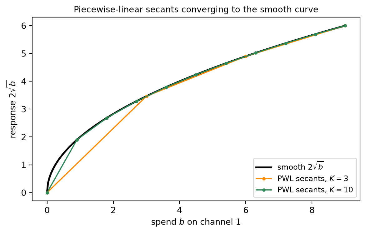
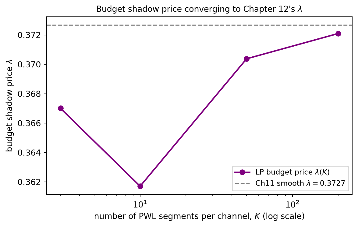
A small example fixes the picture (the full arithmetic is carried out in the Worked Examples and Code Tie-in). Take two channels with decreasing segment slopes [5, 3, 1] and [4, 2, 1], every segment of width 2, and budget B = 5. Filling steepest first pours 2 into the slope-5 segment of channel 1, then 2 into the slope-4 segment of channel 2, then the last 1 into the slope-3 segment of channel 1 — exhausting the budget. The optimal allocation is b^\star = (3, 2), and the marginal (last-funded) segment has slope 3, so the budget shadow price is \lambda = 3. Refining the model brings it back to Chapter 12’s smooth answer: take the square-root responses r_i(b) = a_i\sqrt{b} with a = (2,1) and B = 9, and approximate each by a piecewise-linear concave fit. As the segmentation is refined — more, narrower segments — the LP optimum converges to the smooth concave optimum b^\star = (7.2, 1.8) and the budget shadow price converges to the smooth marginal return \lambda \to 0.3727, exactly the values Chapter 12 produced by the equal-marginal condition.
Finally, the per-channel caps and minimums, when they bind, carry shadow prices of their own. The dual variable on a binding cap \sum_k s_{ik} \le \overline{B}_i is the marginal value of relaxing that cap — how much more total response you could buy by allowing one more dollar into a channel held back at its ceiling. This is multi-constraint duality in plain action: solve the LP once and read off, alongside the budget price \lambda, a separate price for every binding business rule.
Rung 9 — Where linear programming stops
The piecewise-linear-as-LP trick is powerful, and it is bounded. Honesty about a method includes naming where it fails, and this one fails in two distinct ways — one a matter of approximation, the other a matter of structure. Drawing the boundary precisely is what hands the next chapter its job.
It is an approximation. A piecewise-linear curve replaces a smooth response by a chain of straight segments, and the LP optimum is the optimum of the chain, not of the curve. The two differ — but the gap is controllable. Refining the segmentation, using more and narrower segments, makes the piecewise-linear fit hug the smooth curve more tightly, and the LP optimum converges to the true smooth concave optimum as the segment widths shrink. The error is a discretization error, and it goes to zero with the mesh. The Code Tie-in demonstrates exactly this convergence on the square-root example, the refined LP marching to Chapter 12’s (7.2, 1.8) with budget price \lambda \to 0.3727.
It rests entirely on concavity. The deeper limit is structural. The “fill steepest first” rule — and with it the clean vertex optimum, the cutoff slope, the single dual price — is correct only because the slopes decrease. That ordering is what made the exchange argument of Rung 8 go through. Strip away concavity and the whole edifice collapses. Consider Chapter 12’s S-shaped Hill response with exponent n > 1: convex on the toe, concave only past the inflection point. A piecewise-linear fit of such a curve has increasing-then-decreasing slopes — the steepest segments sit in the middle of the curve, not at its start. Filling steepest first is now simply wrong: to reach the lucrative middle segments you may first have to fund the shallow, unprofitable toe, and whether it is worth funding the toe at all is a genuinely discrete, all-or-nothing decision — fund this channel up past its inflection, or skip it entirely. That is an integer decision, and the relaxed problem is non-concave, with the multiple local optima Chapter 12 exhibited. The clean LP structure is gone: such problems belong to integer programming, attacked by branch-and-bound — solving a tree of LP relaxations while branching on the discrete choices — which we note as the discrete tool but do not develop here.
The boundary, stated. Linear programming owns the linear and concave-separable world exactly. There it delivers a global optimum, sitting at a vertex, accompanied by a duality certificate that proves no better point exists — and, as Rung 8 showed, it absorbs the concave budget problem whole, reproducing Chapter 12’s equal-marginal rule as a dual price. The smooth, possibly non-concave world — real saturating, S-shaped channel response — lies outside that boundary. That world is the domain of Chapter 14’s SLSQP, which attacks the nonlinear KKT system directly and iteratively, exactly as Chapter 12 foreshadowed, and which is launched from multiple starting points precisely because the landscape may carry several local optima and no single descent can be trusted to find the global best. Linear programming tells us where optimization is certain; Chapter 14 takes up the terrain where it is merely diligent. That is where the next chapter begins.
Worked Examples
The three steps with the most arithmetic — solving a small LP both graphically and by simplex, reading shadow prices off its dual, and water-filling a piecewise-linear budget — are each small enough to carry out by hand. Working them once fixes what the Fundamental Theorem (Rung 3), the simplex pivots (Rung 4), duality and complementary slackness (Rungs 5–6), and the budget LP (Rung 8) actually deliver. The same two-channel LP threads through Examples 1 and 2, so the primal and its dual can be checked against each other.
Example 1 — A two-variable media LP
Two channels split a budget. Let x_1, x_2 \ge 0 be the spend on each, with constant returns of 3 and 2 per unit. A total budget caps spend at 4, and channel 1 carries its own cap of 2. The plan that maximizes return is the linear program
\max\ 3x_1 + 2x_2 \quad\text{s.t.}\quad x_1 + x_2 \le 4,\ \ x_1 \le 2,\ \ x \ge 0.
(a) Graphically. The two upper bounds and the two nonnegativity constraints cut out a feasible polygon with four vertices: the origin (0,0), the cap corner (2,0), the corner (2,2) where both upper bounds meet, and the budget corner (0,4). The Fundamental Theorem says the optimum sits at one of these corners, so we simply evaluate the objective 3x_1 + 2x_2 at each:
(0,0)\to 0,\qquad (2,0)\to 6,\qquad (2,2)\to 10,\qquad (0,4)\to 8.
The maximum is 10, attained at (2,2) — the Fundamental Theorem made concrete, the optimum landing at a corner rather than in the flat interior. At that corner both constraints x_1 + x_2 \le 4 and x_1 \le 2 bind: spend is at the budget and channel 1 is at its cap.
(b) By simplex. Put the problem in standard form by minimizing the negated objective and adding one slack per inequality:
\min\ -(3x_1 + 2x_2) \quad\text{s.t.}\quad
\begin{aligned}
x_1 + x_2 + s_1 &= 4,\\
x_1 \qquad\;\; + s_2 &= 2,
\end{aligned}
\qquad x, s \ge 0,
with cost vector c = (-3, -2, 0, 0) on (x_1, x_2, s_1, s_2). The slacks give an obvious starting basis B = \{s_1, s_2\} with A_B = I, basic solution (x_1, x_2, s_1, s_2) = (0, 0, 4, 2), and cost 0. We record each pivot as basis, basic solution, entering/leaving choice, and ratio.
Pivot 1. With A_B = I the reduced costs of the nonbasic variables are just their objective coefficients, \bar c_1 = -3 and \bar c_2 = -2. Both are negative, so the vertex is not optimal; the more negative one, x_1, enters. The min-ratio test over the two rows is
t^\star = \min\!\left(\frac{4}{1},\ \frac{2}{1}\right) = 2,
attained in the s_2 row, so s_2 leaves. New basis \{s_1, x_1\}, basic solution (2, 0, 2, 0), cost -6.
Pivot 2. Updating the reduced costs at the new basis, x_2 now carries a negative reduced cost (\bar c_2 = -2 still pays, since raising x_2 uses budget slack s_1, not the exhausted cap), so x_2 enters. The basic variables are x_1 = 2 (held by the cap row) and s_1 = 2 (budget slack); raising x_2 draws down s_1 at rate 1 while leaving x_1 fixed, so the binding ratio is 2/1 = 2 in the s_1 row and s_1 leaves. New basis \{x_2, x_1\}, basic solution (2, 2, 0, 0), cost -10.
Optimality. At \{x_1, x_2\} every reduced cost is now \ge 0 — raising either slack off zero would only add cost — so the test passes and we stop. The optimum is (x_1, x_2) = (2, 2) with objective -(-10) = 10, exactly the graphical answer, reached in two pivots along the edges (0,0) \to (2,0) \to (2,2).
Example 2 — The dual and its shadow prices
Keep the LP of Example 1 and build its dual. Attach a dual variable to each \le constraint: y_1 to the budget x_1 + x_2 \le 4 and y_2 to the cap x_1 \le 2. Reading the primal columns gives one dual constraint per primal variable — the x_1 column (1, 1) with objective coefficient 3, and the x_2 column (1, 0) with coefficient 2:
\min\ 4y_1 + 2y_2 \quad\text{s.t.}\quad y_1 + y_2 \ge 3,\ \ y_1 \ge 2,\ \ y \ge 0.
Solve by complementary slackness. At the primal optimum both variables are positive, x_1 = 2 > 0 and x_2 = 2 > 0, so complementary slackness forces both dual constraints to bind:
y_1 + y_2 = 3, \qquad y_1 = 2 \quad\Longrightarrow\quad y^\star = (2, 1).
Its dual objective is 4(2) + 2(1) = 8 + 2 = 10.
Strong duality. The primal optimum 10 equals the dual optimum 10: the duality gap is exactly zero, precisely as Rung 6 promised, and the matching pair (x^\star, y^\star) certifies that neither can be improved.
Shadow prices. Both primal constraints bind at (2,2), so both dual prices are positive and each is the marginal value of its resource (Rung 7).
- y_1 = 2 is the budget shadow price: one extra unit of budget should raise the objective by 2. Check it directly — relaxing the budget to x_1 + x_2 \le 5 moves the optimum to (2, 3) with value 3(2) + 2(3) = 12, an increase of exactly 2.
- y_2 = 1 is the cap shadow price: one extra unit of channel-1 cap should raise the objective by 1. Relaxing the cap to x_1 \le 3 moves the optimum to (3, 1) with value 3(3) + 2(1) = 11, an increase of exactly 1.
Each dual variable is literally the marginal worth of the resource its constraint rations — solve once, and read off the price of every binding resource.
Example 3 — Allocating a budget over piecewise-linear response
Now the budget LP of Rung 8. Two channels have concave piecewise-linear response: channel 1’s segment slopes are [5, 3, 1] and channel 2’s are [4, 2, 1], every segment has width 2, and the total budget is B = 5. Because the slopes decrease within each channel, the optimum is the water-filling rule — fund the steepest segments first, across both channels, until the budget runs out.
Fill steepest first. Order all six segments by slope:
5\ (\text{ch }1),\quad 4\ (\text{ch }2),\quad 3\ (\text{ch }1),\quad 2\ (\text{ch }2),\quad 1\ (\text{ch }1),\quad 1\ (\text{ch }2).
Pour budget in that order. The slope-5 segment takes its full width 2 (budget used: 2); the slope-4 segment takes its full width 2 (used: 4); the slope-3 segment then takes 1 of its 2 units before the budget hits 5 and stops.
Allocation. Channel 1 received 2 (its slope-5 segment) plus 1 (part of its slope-3 segment) = 3; channel 2 received 2 (its slope-4 segment). So
b^\star = (3, 2), \qquad 3 + 2 = 5 = B.
Total response. Sum slope times width filled over the funded segments:
5\cdot 2 + 3\cdot 1 + 4\cdot 2 = 10 + 3 + 8 = 21.
Budget shadow price. The marginal (last-funded) segment is the slope-3 segment of channel 1, so the budget’s marginal value is \lambda = 3. The water-filling condition checks out: every funded segment has slope \ge 3 (the values 5, 4, 3), and every unfunded segment has slope \le 3 (the slope-3 remainder, then 2, 1, 1). The cutoff slope 3 separates funded from unfunded; one more dollar of budget would buy 3 more units of response by filling more of that slope-3 segment — exactly the shadow price the dual would report.
Tie to Chapter 12. This \lambda = 3 is the discrete equal-marginal return — Chapter 12’s multiplier, here read straight off the LP rather than derived from KKT stationarity. The marginal segments of the active channels share the cutoff slope. And the discreteness is not a limitation: refining a smooth concave response into many narrow segments recovers Chapter 12’s exact answer. For square-root response r_i(b) = a_i\sqrt{b} with a = (2, 1) and B = 9, the refined LP converges to b^\star = (7.2, 1.8) with budget price \lambda \to 0.3727 — the convergence demonstrated in the Code Tie-in.