Motivation
Part IV took the response curve r_i(\cdot) as a given — a smooth function mapping channel i’s spend to the revenue it earns — and built the machinery to optimize over it: convex theory, linear programming, and the production solver SLSQP. The work was real and the results were exact, but one assumption quietly did all the heavy lifting. Nobody asked where the response curve came from. This chapter asks. It writes down the generative model of how a brand’s weekly advertising spend actually produces weekly sales, deriving the curve that Part IV optimized from first principles. That derivation is the data-generating process, and it is the foundation on which everything in Part V rests.
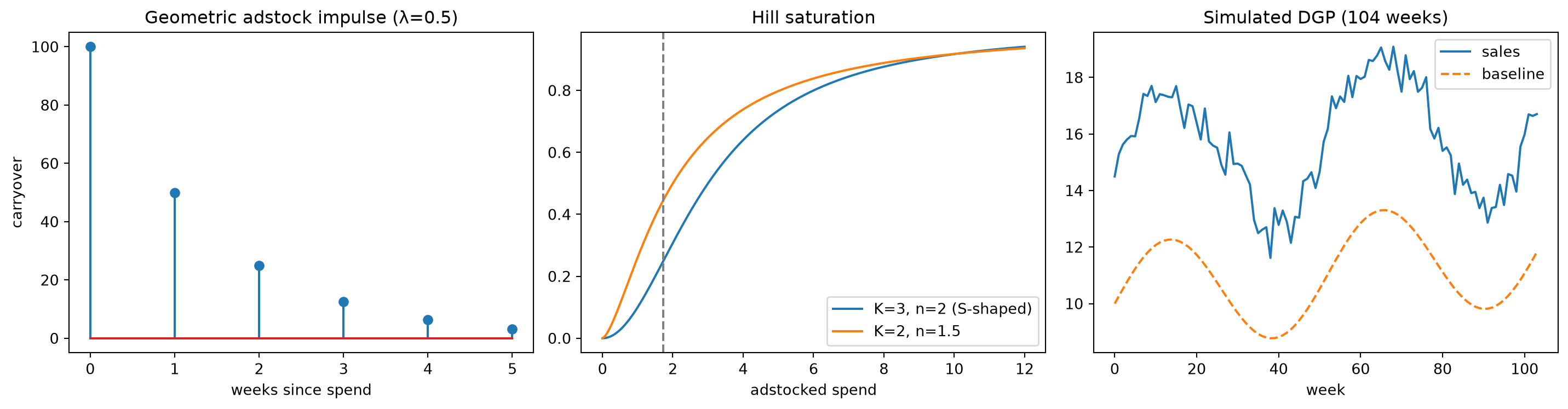
The model has a precise structural form. Weekly sales y_t decompose into three additive pieces: a baseline representing the revenue the brand would have earned even if it had spent nothing on advertising that week — capturing organic demand, seasonality, trend, and all other controls; the incremental contribution of each channel’s spend, passed through two successive nonlinear transforms; and a noise term for everything the model does not explain. That middle piece is where the richness lives. Spend does not translate to sales through a simple scalar multiplier. It passes through two transforms, applied in sequence, that make the relationship nonlinear in both time and amount. Those transforms are the chapter’s stars.
The first transform is adstock, and it captures a mundane fact about advertising: a television spot seen on Monday keeps working on Tuesday, Wednesday, and into the following week as viewers remember and eventually buy. Adstock converts the raw weekly spend x_{i,t} into an effective exposure a_{i,t} by distributing the memory of past spending forward in time — the current effective exposure is a weighted combination of this week’s outlay and the decaying remnants of prior weeks. The second transform is saturation, and it captures an equally mundane fact: the tenth million dollars spent on a channel buys considerably less incremental sales than the first million did. Saturation maps the effective exposure a_{i,t} to a diminishing-returns response s_{i,t} through a nonlinear curve — steep at low exposure and flattening as exposure grows. Trend, seasonality, and control variables are necessary scaffolding, but adstock and saturation are the nonlinear core that gives the model its power and its difficulty.
Once the model has its stars, one sees immediately what Part IV was actually optimizing. The response curve r_i(\cdot) that Chapter 12 took as given is the saturation function evaluated at the adstock-transformed spend — the composed map from raw outlay to incremental sales, its shape determined entirely by the parameters of both transforms. Choosing those parameters is estimation; that is Chapter 16’s work. But first, a harder question arrives. Once we can simulate the data-generating process — once we can generate realistic synthetic spend-and-sales series from a known parameter vector — we can ask whether the reverse journey is possible. Given only the observed spend and the observed sales, can we recover the adstock and saturation parameters that produced them? The answer is no, not from observational spend data alone, and the reason is structural. That identification wound is where this chapter ends, and it is the wound that Part VI heals.
The route through the chapter is as follows. We develop the mathematical form of adstock and saturation, establish their composed action as the channel response function, add the baseline and noise to complete the DGP, and then simulate a fully synthetic week-by-week sales series from a known parameter vector. That synthetic series is the dataset Chapter 16 will fit — a controlled environment where the ground truth is known and the estimation challenge can be examined clearly, before the harder work of fitting to real campaign data.
Theory & Proofs
The theory develops in three steps. Rung 1 states the structural equation, naming every term in the data-generating process. Rung 2 defines adstock — the temporal carryover transform — in its geometric and normalized forms, with a qualitative account of the delayed-peak variant of Jin et al. (2017). Proof P1 then establishes the key identities for geometric adstock: the normalized weights sum to one, a constant input reaches a known steady state, the impulse response decays geometrically, and the half-life and mean lag both reduce to simple closed forms.
Rung 1 — The structural equation
The MMM generative model expresses weekly sales y_t as the sum of four additive pieces:
y_t = \underbrace{\alpha + \tau_t + \sigma_t}_{\text{baseline}} \;+\; \sum_{i=1}^{C} \beta_i\, g\!\big(a_\lambda(x_{i,t})\big) \;+\; \gamma^\top z_t \;+\; \varepsilon_t,
\qquad \varepsilon_t \sim \mathcal{N}(0,\sigma_\varepsilon^2).
The baseline groups three terms: \alpha is a fixed intercept representing average organic revenue, \tau_t is a slow trend capturing long-run brand growth or decline (commonly a spline or linear drift), and \sigma_t is a periodic seasonality component — a yearly cycle is the most common. These terms set the revenue floor the brand earns in the absence of paid advertising. The media contribution sums over all C channels: x_{i,t} is channel i’s spend in week t, the transform a_\lambda converts that spend into an effective exposure by distributing the memory of past outlays across time, g then compresses the resulting exposure through a diminishing-returns saturation curve, and \beta_i > 0 scales the compressed response into revenue units. The composed map g \circ a_\lambda is the channel response curve that Part IV optimized; its parameters — the adstock decay and the saturation shape — are what estimation must recover. The vector z_t collects exogenous controls such as price indices or holiday indicators, with coefficient vector \gamma; and \varepsilon_t \sim \mathcal{N}(0,\sigma_\varepsilon^2) absorbs unexplained variation.
The non-media terms are kept deliberately simple here. Their functional form matters far less than the fact that they share variance with spend: organic sales tend to rise during periods of heavy advertising investment, seasonal peaks often coincide with campaign flights, and price promotions run alongside elevated media pressure. That collinearity is the confounding structure examined later in the chapter; for now, including these terms even in simplified form ensures the DGP captures the variance-sharing that makes identification difficult.
Rung 2 — Adstock and carryover
Advertising exposure is not instantaneous. A viewer who sees a television spot on Monday may not buy until Friday; word-of-mouth from a campaign spreads across weeks; repeated exposures build recall that persists after spending stops. Adstock formalizes this memory by replacing the raw weekly outlay x_{i,t} with an effective exposure that blends current spend with the decaying remnants of the past.
Geometric adstock. The simplest and most widely used specification is the geometric filter with decay parameter \lambda \in [0,1), defined equivalently by a recursion and by its infinite-sum expansion:
a_\lambda(x)_t \;=\; x_t + \lambda\, a_\lambda(x)_{t-1} \;=\; \sum_{k=0}^{\infty} \lambda^k x_{t-k}, \qquad \lambda \in [0,1).
Unrolling the recursion one step at a time reproduces the infinite weighted sum; the weights \lambda^k decay geometrically with lag k. When \lambda = 0 the adstock reduces to raw spend; as \lambda \to 1 the memory lengthens and the filter becomes increasingly persistent.
Normalized form. Define the weights w_k = (1-\lambda)\lambda^k for k = 0, 1, 2, \ldots. These sum to unity — Proof P1 establishes this from the geometric series — so the normalized adstock \tilde{a}_\lambda(x)_t = \sum_{k=0}^{\infty} w_k\, x_{t-k} is a proper weighted moving average. Normalized adstock preserves the level of a constant input: x_t \equiv x implies \tilde{a}_\lambda(x)_t = x for all t. This makes the coefficient \beta_i directly interpretable as marginal revenue per unit of spend, not per unit of accumulated effective exposure.
Delayed-peak adstock. The geometric filter places maximum weight at lag k = 0 and decays monotonically thereafter — carryover is largest the week of the spend and strictly diminishes from there. The delayed-peak variant of Jin et al. (2017) relaxes this by allowing the impulse-response weights to rise from zero, reach a peak a few lags out, and then decay, capturing campaigns that build awareness over repeated exposures before they fade. This shape requires two parameters rather than one and its analysis follows a different path; Proof P1 covers only the geometric case.
Proof P1 — Geometric adstock identities
Proposition P1. Let \lambda \in [0, 1), define a_\lambda(x)_t = \sum_{k=0}^{\infty} \lambda^k x_{t-k}, and let w_k = (1-\lambda)\lambda^k. Then: (i) \sum_{k=0}^{\infty} w_k = 1; (ii) constant input x_t \equiv x gives unnormalized adstock x/(1-\lambda) and normalized adstock x; (iii) the impulse x_0 = 1, x_t = 0 for t \neq 0, gives a_\lambda(x)_t = \lambda^t with total mass 1/(1-\lambda); (iv) the half-life is t_{1/2} = \log_\lambda \tfrac{1}{2}; (v) the mean lag is \bar{k} = \lambda/(1-\lambda).
Proof.
(i) Normalization. The weights form a geometric series with first term (1-\lambda) and ratio \lambda. Since |\lambda| < 1 the series converges:
\sum_{k=0}^{\infty} w_k = (1-\lambda) \sum_{k=0}^{\infty} \lambda^k = (1-\lambda) \cdot \frac{1}{1-\lambda} = 1.
The weights therefore constitute a valid probability distribution on the nonnegative integers. In particular, constant input x_t \equiv x gives normalized adstock \tilde{a}_\lambda(x)_t = x \sum_{k=0}^{\infty} w_k = x: the level is preserved exactly.
(ii) Unnormalized steady state. For constant x_t \equiv x, the unnormalized filter gives
a_\lambda(x)_t = \sum_{k=0}^{\infty} \lambda^k x = x \sum_{k=0}^{\infty} \lambda^k = \frac{x}{1-\lambda}.
The factor 1/(1-\lambda) > 1 is the steady-state amplification: a channel spending x every week accumulates effective exposure x/(1-\lambda). At \lambda = 0.5 this is 2x.
(iii) Impulse response. Set x_0 = 1 and x_t = 0 for t \neq 0. Only the k = t term survives in the sum, so a_\lambda(x)_t = \lambda^t \cdot 1 = \lambda^t for t \geq 0. The total mass is
\sum_{t=0}^{\infty} \lambda^t = \frac{1}{1-\lambda},
matching the steady-state amplification of (ii): both expressions measure the filter’s total weight.
(iv) Half-life. The impulse response at lag t is \lambda^t. The half-life t_{1/2} satisfies \lambda^{t_{1/2}} = 1/2; taking logarithms:
t_{1/2} \ln \lambda = \ln \tfrac{1}{2} \implies t_{1/2} = \frac{\ln(1/2)}{\ln \lambda} = \log_\lambda \tfrac{1}{2}.
Since \ln \lambda < 0 and \ln(1/2) < 0, the ratio is positive. At \lambda = 0.5: t_{1/2} = \ln 2 / \ln 2 = 1 week.
(v) Mean lag. The mean lag under the normalized weight distribution is
\bar{k} = \sum_{k=0}^{\infty} k\, w_k = (1-\lambda) \sum_{k=0}^{\infty} k \lambda^k.
Differentiating the geometric-series identity \sum_{k=0}^{\infty} \lambda^k = 1/(1-\lambda) term by term with respect to \lambda gives \sum_{k=1}^{\infty} k \lambda^{k-1} = 1/(1-\lambda)^2; multiplying by \lambda yields \sum_{k=0}^{\infty} k \lambda^k = \lambda/(1-\lambda)^2. Substituting:
\bar{k} = (1-\lambda) \cdot \frac{\lambda}{(1-\lambda)^2} = \frac{\lambda}{1-\lambda}.
At \lambda = 0.5: \bar{k} = 0.5 / 0.5 = 1 week.
Summary at \lambda = 0.5. The three summary statistics coincide: the half-life is 1 week, the mean lag is 1 week, and the steady-state amplification is 2x. This trio provides a rapid calibration check — to model roughly one week of carryover, initialize \lambda = 0.5 and adjust as the data indicate. \blacksquare
Rung 3 — Saturation and shape
The saturation transform maps effective exposure to a dimensionless response bounded strictly between zero and one. The Hill curve — long used in dose–response modeling — accomplishes this with two parameters:
g(x;\, K,\, n) = \frac{x^{n}}{K^{n} + x^{n}}, \qquad x \ge 0,\; K > 0,\; n > 0.
The parameter K is the half-saturation point: direct substitution gives g(K) = K^n / (K^n + K^n) = \tfrac{1}{2}, so spend equal to K earns exactly half the maximum possible response. The parameter n controls steepness and shape: for n \le 1 the curve rises steeply at the origin and flattens immediately, while for n > 1 it begins nearly flat — a convex toe — before bending into its familiar diminishing-returns arc. This is the very curve Chapters 12–14 optimized over; it is defined here at last from the model’s first principles.
Proof P2 — Hill shape theorem
Proposition P2. For x > 0, K > 0, n > 0, the Hill function g(x;\,K,n) = x^n/(K^n + x^n) is strictly increasing and bounded in (0,1), with g(0^+) = 0, g(\infty) = 1, and g(K) = \tfrac{1}{2}. For n \le 1, g is concave on (0,\infty). For n > 1, g has a single inflection at x^\star = K\big(\tfrac{n-1}{n+1}\big)^{1/n}, is convex on (0, x^\star), and concave on (x^\star, \infty).
Proof.
Monotone and bounded. Differentiating with the quotient rule and collecting:
g'(x) = \frac{n x^{n-1}(K^n + x^n) - x^n \cdot n x^{n-1}}{(K^n + x^n)^2} = \frac{n K^n x^{n-1}}{(K^n + x^n)^2}.
Every factor in the numerator is positive for x > 0, so g'(x) > 0: g is strictly increasing. As x \to 0^+ the numerator x^n \to 0 while the denominator approaches K^n, giving g(0^+) = 0; as x \to \infty, x^n dominates K^n + x^n, giving g(\infty) = 1. At x = K the numerator and denominator are equal, so g(K) = K^n/(2K^n) = \tfrac{1}{2}.
Curvature. Differentiating g'(x) = nK^n x^{n-1}(K^n + x^n)^{-2} by the product rule and simplifying yields:
g''(x) = \frac{nK^n x^{n-2}}{(K^n + x^n)^3}\Big[(n-1)K^n - (n+1)x^n\Big].
The prefactor \dfrac{nK^n x^{n-2}}{(K^n+x^n)^3} is strictly positive for x > 0, so \operatorname{sign} g'' = \operatorname{sign}\big[(n-1)K^n - (n+1)x^n\big].
Case n \le 1. When n < 1 the term (n-1)K^n is negative and -(n+1)x^n is also negative, so their sum is negative for all x > 0. When n = 1 the bracket reduces to 0 - 2x^n < 0. In both sub-cases g'' < 0 everywhere: g is concave on (0,\infty), delivering diminishing returns from the first dollar.
Case n > 1. Here (n-1) > 0, so the bracket (n-1)K^n - (n+1)x^n is positive at small x and decreasing. Setting it to zero:
(n-1)K^n = (n+1)x^n \implies x^\star = K\!\left(\frac{n-1}{n+1}\right)^{\!1/n}.
For x < x^\star the bracket is positive (g'' > 0: convex); for x > x^\star it is negative (g'' < 0: concave). Since the bracket is strictly decreasing in x^n, this zero is unique.
Numeric anchor (K = 3, n = 2). The inflection is at x^\star = 3\cdot(1/3)^{1/2} = \sqrt{3} \approx 1.732. Evaluating: g(\sqrt{3}) = 3/(9 + 3) = 0.25; g(3) = 9/18 = 0.5; g'(3) = 2\cdot9\cdot3/(18)^2 = 54/324 = \tfrac{1}{6}; g'(\sqrt{3}) = 2\cdot9\cdot\sqrt{3}/(12)^2 = 18\sqrt{3}/144 = \tfrac{\sqrt{3}}{8}.
This is the concavity Part IV assumed when it invoked equal-marginal allocation; for n > 1 the convex toe — the region below x^\star where marginal returns are still rising — is precisely why Chapters 12–14 had to guard against non-convexity. \blacksquare
Rung 4 — Assembling the DGP
The per-channel data-generating pipeline runs in a fixed sequence: raw spend x_{i,t} passes through the adstock filter to produce effective exposure, which passes through the saturation curve to produce a dimensionless response, which is scaled by \beta_i and summed across channels i = 1, \ldots, C; baseline, controls, and noise are then added as in Rung 1. The canonical formulation of Jin et al. (2017) applies adstock first, then saturation — the composition g \circ a_\lambda — and this ordering is a genuine modeling choice, not a convention: Proof P3 shows that reversing it produces a numerically different model.
Proof P3 — Non-commutativity of adstock and saturation
Proposition P3. In general, (g \circ a_\lambda)(x) \neq (a_\lambda \circ g)(x): adstock-then-saturate and saturate-then-adstock produce different time series.
Proof. We construct an explicit numeric counterexample. Let the spend sequence be x_0 = 3, x_1 = 0, with decay \lambda = 0.5, half-saturation K = 3, and shape n = 2.
Path 1 — adstock then saturate. Apply the adstock filter first. At t = 0: a_0 = x_0 = 3. At t = 1: a_1 = x_1 + \lambda\, a_0 = 0 + 0.5 \cdot 3 = 1.5. The effective-exposure sequence is (3,\; 1.5). Applying saturation term by term:
g(3) = \frac{3^2}{3^2 + 3^2} = \frac{9}{18} = 0.5, \qquad g(1.5) = \frac{1.5^2}{3^2 + 1.5^2} = \frac{2.25}{11.25} = 0.2.
The saturated sequence under Path 1 is (0.5,\; 0.2).
Path 2 — saturate then adstock. Apply saturation to the raw spend first:
g(3) = 0.5, \qquad g(0) = \frac{0^2}{3^2 + 0^2} = 0.
The pre-saturated sequence is (0.5,\; 0). Applying the adstock filter: at t = 0 the output is 0.5; at t = 1 the output is 0 + 0.5 \cdot 0.5 = 0.25. The adstocked sequence under Path 2 is (0.5,\; 0.25).
Comparison. At the impulse period t = 0 both paths agree: 0.5 = 0.5. At the carryover period t = 1 they differ: 0.2 \neq 0.25. The disagreement lives entirely in the carryover period — Path 1 carries forward the compressed (saturated) effective exposure, while Path 2 carries forward raw spend and then compresses. Because the saturation function is nonlinear, carrying over a compressed signal is not equivalent to compressing a carried-over signal. The ordering of transforms is therefore a modeling decision with empirical consequences. \blacksquare
Rung 5 — The identification wound
With the DGP assembled, a natural question surfaces: given an observed time series of weekly spend and weekly sales (x_{i,t}, y_t), can the parameters (\beta_i, K, n, \lambda) governing channel i’s response be recovered from the data? The answer, under realistic observational conditions, is no — not without additional information beyond what any ordinary campaign budget provides. Three structural features of advertising data conspire to make the inverse problem ill-posed.
The first is operating-range confinement. Firms do not randomize their budgets. A brand that has run a given channel at roughly the same level for two years has produced data that cluster near a single operating point on the saturation curve. The observed (x_{i,t}, y_t) pairs constrain what the response function looks like near that point; they say almost nothing about its shape at other spend levels. The consequence is that many different curves — steep ones, flat ones, curves peaking early, curves with a delayed inflection — can all fit the same narrow band of observed data equally well.
The second is cross-channel collinearity. Marketing budgets are governed by planning cycles, seasonal flights, and product launches, not set independently by channel. Television, digital, and radio spend tend to rise and fall together. When several channels are highly correlated, the model cannot attribute a given week’s sales lift to any one channel versus the others. The summed contribution \sum_{i=1}^{C} \beta_i g(a_\lambda(x_{i,t})) may be well determined, but the individual \beta_i are not: infinitely many allocations of credit across channels can produce the same fitted values.
The third is baseline confounding. Firms spend more on advertising during high-demand periods — a holiday quarter, a product launch, a competitor’s exit — precisely because the expected return is higher. The baseline term \alpha + \tau_t + \sigma_t captures the same demand variation that is also driving spend upward. A model that cannot distinguish the organic demand surge from the advertising effect will attribute too much of the observed sales lift to media. In the structural equation of Rung 1 this ambiguity is explicit: the baseline and the media contributions share variance by construction, and without exogenous leverage on spend neither can be pinned down separately.
These three pathologies interact and reinforce each other in practice. But even in the cleanest possible case — a single channel, no collinearity, baseline fully controlled — operating-range confinement alone is sufficient to make the saturation parameters non-identifiable. Proof P4 establishes this in the sharpest possible form.
Proof P4 — Non-identifiability at a single operating point
Proposition P4. Suppose channel i’s spend is observed only at a single operating point x_0, so the data constrain the model only through the scalar \beta_i\, g(x_0;\, K, n). Then the parameters (\beta_i, K, n) are not identified: distinct parameter vectors exist that are observationally indistinguishable on the support \{x_0\}.
Proof. Fix x_0 = 3 and n = 2 throughout. For any parameter vector (\beta_i, K, n), the observable channel contribution at x_0 is
c = \beta_i\, g(3;\, K,\, 2) = \beta_i \cdot \frac{9}{K^2 + 9}.
We exhibit two distinct parameter vectors that both give c = 0.5.
Parameter set A. Take (\beta_i, K, n) = (1,\, 3,\, 2). Then
g(3;\, 3,\, 2) = \frac{3^2}{3^2 + 3^2} = \frac{9}{18} = 0.5,
and the channel contribution is 1 \cdot 0.5 = 0.5.
Parameter set B. Take (\beta_i, K, n) = (2,\, 3\sqrt{3},\, 2). Note 3\sqrt{3} \approx 5.196. Then
g\!\left(3;\, 3\sqrt{3},\, 2\right) = \frac{3^2}{\left(3\sqrt{3}\right)^2 + 3^2} = \frac{9}{27 + 9} = \frac{9}{36} = 0.25,
and the channel contribution is 2 \cdot 0.25 = 0.5.
The ridge. Both parameter vectors produce identical expected sales at x_0 = 3:
1 \cdot g(3;\, 3,\, 2) \;=\; 0.5 \;=\; 2 \cdot g\!\left(3;\, 3\sqrt{3},\, 2\right).
Because the observable is the single number c = \beta_i\, g(x_0;\, K, n), the likelihood as a function of (\beta_i, K, n) is flat along the ridge \{ (\beta_i, K) : \beta_i \cdot 9 / (K^2 + 9) = 0.5 \} for fixed n = 2. No accumulation of data gathered at x_0 = 3 — not more weeks, not smaller measurement error — can distinguish Set A from Set B, because all such observations are identical draws from the same likelihood.
Identifying the shape parameters (K, n) — not merely the height of the curve at a single point — requires spend that varies across a non-trivial range of the saturation curve. When the regressor is confined to a support of lower dimension than the parameter count, the likelihood is flat along a manifold, and estimation recovers only the composite \beta_i\, g(x_0;\, K, n), never the factors separately. \blacksquare
Breaking this degeneracy requires exogenous variation in spend — randomized or quasi-experimental shifts in the operating point that observational budgets cannot supply — and that is exactly the leverage Part VI (Chapters 19–22) provides.
Worked Examples
Three calculations carry the chapter’s main results into arithmetic — one for each structural component of the data-generating process. The first runs the geometric adstock recursion by hand and reads off the three summary statistics of Proof P1: half-life, mean lag, and steady-state amplification. The second maps the Hill curve at the parameter pair that anchored Part IV, recovering the inflection and marginals of Proof P2 as explicit numbers. The third exhibits two parameter pairs that are observationally indistinguishable at a single spend level, instantiating the identification manifold of Proof P4 with a pair of two-line verifications.
WE1 — Geometric adstock by hand
Set \lambda = 0.5 and supply the four-week spend sequence [100, 0, 0, 0] — a single impulse of 100 in week 0 followed by silence. The recursion a_t = x_t + \lambda\, a_{t-1} (with a_{-1} = 0) runs as follows.
Week 0. a_0 = x_0 + 0.5 \cdot 0 = 100.
Week 1. a_1 = x_1 + 0.5 \cdot a_0 = 0 + 0.5 \cdot 100 = 50.
Week 2. a_2 = x_2 + 0.5 \cdot a_1 = 0 + 0.5 \cdot 50 = 25.
Week 3. a_3 = x_3 + 0.5 \cdot a_2 = 0 + 0.5 \cdot 25 = 12.5.
The effective-exposure sequence is [100, 50, 25, 12.5] — precisely the geometric decay 100 \cdot (0.5)^t that Proof P1’s impulse-response identity predicts.
Three summary statistics follow directly from \lambda = 0.5.
Half-life. The decay reaches half its initial value when (0.5)^{t_{1/2}} = 1/2, so
t_{1/2} = \frac{\ln(1/2)}{\ln(0.5)} = \frac{-\ln 2}{-\ln 2} = 1 \text{ week}.
Mean lag. Under the normalized weights w_k = (1-\lambda)\lambda^k, the expected lag is
\bar{k} = \frac{\lambda}{1-\lambda} = \frac{0.5}{0.5} = 1 \text{ week}.
For \lambda = 0.5 the half-life and mean lag coincide — a coincidence specific to this value.
Steady state. A channel spending 100 every week builds up accumulated exposure until inflow and decay balance. Proof P1 part (ii) gives the unnormalized steady state x/(1-\lambda):
a_\infty = \frac{100}{1 - 0.5} = 200.
Sustained weekly spend of 100 produces an effective exposure of 200 — the saturation function receives 200 as its argument, not 100. The two-week amplification at \lambda = 0.5 is why evaluating a campaign after only one week understates its eventual contribution; the accumulation has not yet reached equilibrium.
WE2 — The Hill curve at K = 3, n = 2
With half-saturation K = 3 and shape n = 2, the Hill curve is g(x) = x^2/(9 + x^2). Four quantities pin down its shape.
At the half-saturation point. By definition g(K) = \tfrac{1}{2}; direct substitution confirms it:
g(3) = \frac{3^2}{3^2 + 3^2} = \frac{9}{18} = 0.5.
At the inflection. Proof P2 locates the inflection at x^\star = K\bigl((n-1)/(n+1)\bigr)^{1/n}. Substituting K = 3 and n = 2:
x^\star = 3\!\left(\frac{1}{3}\right)^{\!1/2} = \frac{3}{\sqrt{3}} = \sqrt{3} \approx 1.732.
Its height is
g\!\left(\sqrt{3}\right) = \frac{\left(\sqrt{3}\right)^2}{3^2 + \left(\sqrt{3}\right)^2} = \frac{3}{9 + 3} = \frac{3}{12} = 0.25.
The curve crosses one quarter of its maximum response at the inflection, well below the half-saturation level.
Marginals. The derivative formula from Proof P2 is g'(x) = nK^n x^{n-1}/(K^n + x^n)^2. At the half-saturation point:
g'(3) = \frac{2 \cdot 9 \cdot 3}{(9 + 9)^2} = \frac{54}{324} = \frac{1}{6} \approx 0.167.
At the inflection:
g'\!\left(\sqrt{3}\right) = \frac{2 \cdot 9 \cdot \sqrt{3}}{(9 + 3)^2} = \frac{18\sqrt{3}}{144} = \frac{\sqrt{3}}{8} \approx 0.217.
The marginal return is higher at the inflection than at the half-saturation point — the curve is still accelerating below x^\star and decelerating above it, so the steepest slope lives precisely at the inflection.
Closing the loop. This is the exact curve whose shape Part IV optimized. The region x < \sqrt{3} where g'' > 0 is the convex toe that forced Chapters 12–14 to guard against non-concavity; x^\star = \sqrt{3} is the inflection Chapter 12 cited without derivation. Proof P2 has now closed that gap: the inflection formula delivers \sqrt{3} directly, and Part V has derived the object Part IV had to take on faith.
WE3 — Non-identifiability made concrete
A single operating point constrains the value of \beta \cdot g(x_0;\, K, n) at one argument — it does not constrain the individual factors. Fix x_0 = 3, n = 2, and suppose the data yield a channel contribution of 0.5 at that spend level. Two distinct parameter pairs, both with n = 2, reproduce the observation exactly.
Parameter pair A: (\beta, K) = (1, 3).
\beta \cdot g(x_0;\, K,\, 2) = 1 \cdot \frac{3^2}{3^2 + 3^2} = 1 \cdot \frac{9}{18} = 0.5.
Parameter pair B: (\beta, K) = (2,\, 3\sqrt{3}). Note (3\sqrt{3})^2 = 27, so
\beta \cdot g\!\left(x_0;\, 3\sqrt{3},\, 2\right) = 2 \cdot \frac{3^2}{(3\sqrt{3})^2 + 3^2} = 2 \cdot \frac{9}{27 + 9} = 2 \cdot \frac{9}{36} = 2 \cdot 0.25 = 0.5.
Both pairs give exactly 0.5. Pair A uses a curve with K = 3: spend x_0 = 3 sits at its half-saturation point. Pair B uses a curve with K = 3\sqrt{3} \approx 5.2: spend x_0 = 3 sits below its half-saturation point, but the larger scale \beta = 2 exactly compensates. Any number of weeks of data at x_0 = 3 cannot separate these two stories, because every observation is an identical draw from the same likelihood: the data constrain only the product \beta \cdot g(3;\, K, 2), never \beta and K individually.
The fix is not more data at x_0 = 3 — it is data at other spend levels. Points drawn from the steep lower region and from the flat upper region of the saturation curve force the curve’s shape, pinning K and releasing \beta separately. That variation is absent from an ordinary budget held roughly constant; obtaining it requires deliberate experimental variation in spend spread across a meaningful range of the saturation curve. This is the wound Proof P4 put on record, and the leverage Part VI (Chapters 19–22) provides.