Theory & Proofs
The five rungs develop from the most foundational result outward. Rung 1 establishes the calibration likelihood in full generality and keys every term to Chapter 20’s taxonomy. Rung 2 proves the keystone compression result: a calibration factor on a linear functional of the parameters is a rank-one precision update, and the variance reduction is largest where the observational precision is smallest — the ridge heals. Rung 3 proves the secant–tangent matching theorem, which governs how a finite lift test’s secant is related to the tangent the optimizer needs, and derives the paired-bracketing correction. Rung 4 develops the identification geometry: how many constraints of what types are needed to pin the curve’s shape parameters. Rung 5 introduces power-prior down-weighting and connects the accumulated system of weighted calibration factors to the prior store of Chapter 22.
Rung 1 — The calibration likelihood factor (taxonomy-keyed). Bayesian evidence synthesis treats an experimental estimate \hat g as a noisy observation of a functional g(\theta) of the response-curve parameters, incorporating it through the standard likelihood factorization. The joint posterior on \theta given both the observational MMM data D and the experimental estimate \hat g is:
p(\theta \mid D, \hat g) \;\propto\; p(\theta)\,\underbrace{L_{\text{obs}}(\theta\mid D)}_{\text{the MMM fit}}\,\underbrace{L_{\text{exp}}(\hat g \mid \theta)}_{\text{calibration factor}} .
The observational likelihood L_{\text{obs}} is the standard MMM likelihood — the probability of the observed sales series under the fitted response-curve parameters. The calibration factor L_{\text{exp}} encodes what the experiment learned about the parameters, and its precise form depends on which entry in Chapter 20’s taxonomy the experiment produced.
- Secant: The experiment measured a lift \hat\Delta over the spend interval [x, x+\delta]. Since S(x+\delta;\theta) - S(x;\theta) is the true lift implied by the model, the factor is \hat\Delta \mid \theta \sim \mathcal N\!\big(S(x{+}\delta;\theta) - S(x;\theta),\, s^2\big), where s^2 is the experimental variance. When lifts are constrained to be positive a Gamma calibration factor is the practical variant: it respects the positivity boundary while retaining conjugate-like tractability near the mode.
- Tangent: The experiment measured something proportional to the marginal return at a single operating point x — for example, a regression-discontinuity estimate. The factor becomes \widehat{S'}\cdot\delta \mid \theta \sim \mathcal N\!\big(S'(x;\theta)\,\delta,\, s^2\big), matching the marginal scaled by the test displacement.
- Validation: A holdout forecast check or a non-revenue awareness lift that constrains forecast accuracy rather than any parameter of S provides no likelihood term at all. It enters as a posterior-predictive check — a conflict alarm that warns if the observational and experimental distributions are inconsistent, but does not update the response-curve parameters.
The critical observation is that the experiment is information about a functional of \theta, not about \theta directly. Inserting it as a likelihood factor composes cleanly with the observational likelihood in the product above, exploiting no data twice: L_{\text{obs}} was formed from the time series D, and L_{\text{exp}} was formed from a separate randomization. This is the precise sense in which the experimental estimate is cleaner than re-expressing it as a prior on a derived quantity: a prior conflates uncertainty about the functional with uncertainty about everything else, and adjusting the prior to match the experiment collapses the distinction between “the data say” and “I believe.”
Rung 2 — Proof P1 (KEYSTONE): a calibration factor compresses the posterior in the constrained direction (the ridge heals). Consider the linear-Gaussian setting in which the observational posterior on \theta \in \mathbb{R}^d is \theta \mid D \sim \mathcal N(m_{\text{obs}}, \Lambda_{\text{obs}}^{-1}), and a calibration experiment measures a linear functional c^\top\theta with noise: \hat g \mid \theta \sim \mathcal N(c^\top\theta,\, s^2). The following theorem identifies the posterior precision after incorporating the calibration factor.
Theorem. The posterior precision matrix after Bayesian evidence synthesis is
\Lambda_{\text{post}} = \Lambda_{\text{obs}} + \tfrac{1}{s^2}\,c\,c^\top .
Proof. The log-posterior is the sum of the observational log-posterior and the calibration log-likelihood:
\log p(\theta \mid D, \hat g) = -\tfrac{1}{2}(\theta - m_{\text{obs}})^\top \Lambda_{\text{obs}} (\theta - m_{\text{obs}}) - \tfrac{1}{2s^2}(\hat g - c^\top\theta)^2 + \text{const}.
Expanding the calibration quadratic in \theta: (\hat g - c^\top\theta)^2 = \hat g^2 - 2\hat g\,c^\top\theta + \theta^\top(cc^\top)\theta. Collecting all second-order terms in \theta across both quadratics, the coefficient of -\tfrac{1}{2}\theta^\top(\cdot)\theta is
\Lambda_{\text{obs}} + \tfrac{1}{s^2}\,c\,c^\top ,
which is the posterior precision (the negative Hessian of the log-posterior). The posterior is therefore Gaussian with this precision matrix: \theta \mid D, \hat g \sim \mathcal N(m_{\text{post}}, \Lambda_{\text{post}}^{-1}) where \Lambda_{\text{post}} = \Lambda_{\text{obs}} + \tfrac{1}{s^2}cc^\top — a rank-one update, adding a single dyadic \tfrac{1}{s^2}cc^\top to the observational precision. For the variance along the direction c: projecting onto the unit vector \hat c = c/\lVert c\rVert and applying the Sherman–Morrison identity, the posterior variance in direction \hat c falls from (\hat c^\top \Lambda_{\text{obs}} \hat c)^{-1} to (\hat c^\top \Lambda_{\text{obs}} \hat c + \lVert c\rVert^2 / s^2)^{-1}. Writing the observational precision in direction \hat c as \Lambda_{\text{obs},c} = \hat c^\top \Lambda_{\text{obs}} \hat c, the posterior precision in that direction is \Lambda_{\text{obs},c} + \lVert c\rVert^2/s^2, a strict increase: the variance is strictly reduced. The relative variance reduction is largest where \Lambda_{\text{obs},c} is smallest — precisely the near-null directions of \Lambda_{\text{obs}}, the identifiability ridge. \blacksquare
MMM reading. The Chapter 16 Fisher-information ridge is the near-flat eigendirection of \Lambda_{\text{obs}}: the direction in parameter space that the observational spend data barely excite, because historical spend variation was never designed to isolate counterfactual channel contrasts. A Chapter 20 experiment aimed at that contrast direction supplies precisely the missing precision through the rank-one update, and the Chapter 18 allocation posterior — wide because of the ridge — narrows in direct proportion to the calibration factor’s precision. The EVPI gap, measuring the value of resolving parameter uncertainty before committing to an allocation, shrinks accordingly.
Anchor. Along the attribution contrast direction u = (1,-1)/\sqrt{2} (so \lVert c\rVert^2 = 1), take observational precision \Lambda_{\text{obs},c} = 1 (variance 1, std 1). A calibration factor with measurement precision 1/s^2 = 3 gives posterior precision \Lambda_{\text{obs},c} + \lVert c\rVert^2/s^2 = 1 + 3 = 4, posterior variance 0.25, posterior std 0.5. The ridge standard deviation halves (from 1 to 0.5) and its variance drops 4\times (from 1 to 0.25) — the precision ratio \Lambda_{\text{post}}/\Lambda_{\text{obs}} = 4 governs the variance reduction directly.
Rung 3 — Proof P2 (KEYSTONE): the secant–tangent matching relationship. A finite lift test measures a secant — the average slope of S over the tested spend interval. The optimizer of Chapter 18, however, needs the tangent S'(x) at the current operating spend. These two quantities are related by the second-order Taylor expansion of S, and the mismatch between them is an O(\delta) bias under concavity that a paired bracketing design can correct.
Theorem (Taylor with remainder). For S \in C^2, the secant over an interval of length \delta starting at x equals the tangent at x plus a curvature correction:
\frac{S(x{+}\delta)-S(x)}{\delta} = S'(x) + \frac{\delta}{2}\,S''(\xi), \qquad \xi\in(x,x{+}\delta) .
Under strict concavity (S'' < 0), the secant strictly underestimates the lower-endpoint tangent S'(x) by \tfrac{\delta}{2}|S''(\xi)| — a bias of order O(\delta).
Corollary (paired bracketing). Averaging matched up-test and down-test one-sided secants about x cancels the O(\delta) term and achieves second-order accuracy:
\frac{1}{2}\!\left(\frac{S(x{+}\delta)-S(x)}{\delta}+\frac{S(x)-S(x{-}\delta)}{\delta}\right)=S'(x)+O(\delta^2) .
Proof. The first display is Taylor’s theorem with Lagrange remainder: S(x+\delta) = S(x) + \delta S'(x) + \tfrac{\delta^2}{2}S''(\xi) for some \xi \in (x, x+\delta); rearranging gives the stated identity. For the corollary, expand both one-sided secants to third order: S(x \pm \delta) = S(x) \pm \delta S'(x) + \tfrac{\delta^2}{2}S''(x) \pm \tfrac{\delta^3}{6}S'''(x) + O(\delta^4). The forward and backward one-sided secants are then
\begin{aligned}
\frac{S(x+\delta)-S(x)}{\delta} &= S'(x) + \tfrac{\delta}{2}S''(x) + O(\delta^2), \\
\frac{S(x)-S(x-\delta)}{\delta} &= S'(x) - \tfrac{\delta}{2}S''(x) + O(\delta^2),
\end{aligned}
and their average is S'(x) + O(\delta^2): the first-order curvature terms \pm\tfrac{\delta}{2}S''(x) cancel by sign symmetry, leaving only the O(\delta^2) residual. \blacksquare
Anchors. For S = 2\sqrt{x}, x = 4, \delta = 5: secant [S(9)-S(4)]/5 = 2/5 = 0.4; tangent S'(4) = 0.5; gap 0.4 - 0.5 = -0.1. The curvature correction satisfies S''(\xi)\cdot\delta/2 = -0.1, giving S''(\xi) = -0.04; solving S''(\xi) = -1/(2\xi^{3/2}) = -0.04 yields \xi \approx 5.39 \in (4, 9), confirming the Lagrange remainder. For the paired bracketing about x = 9, \delta = 4: the up-secant [S(13)-S(9)]/4 = (2\sqrt{13}-6)/4 \approx 0.303, the down-secant [S(9)-S(5)]/4 = (6-2\sqrt{5})/4 \approx 0.382, their average \approx 0.342 against the tangent S'(9) = 1/3 \approx 0.333. Each individual secant is off by approximately 0.04; the average is off by only 0.009, demonstrating the second-order accuracy gain from the symmetric design.
Rung 4 — Identification: test design \leftrightarrow curve shape. A saturating response curve is generally described by multiple shape parameters. In the Hill form, the general saturating curve is S(x;\theta,\kappa,\alpha) = \theta \cdot x^\alpha / (\kappa^\alpha + x^\alpha), with a scale \theta, a half-saturation point \kappa, and a shape exponent \alpha. One calibration constraint — a single secant or tangent measurement — pins only one functional of (\theta,\kappa,\alpha): a scalar equation in three unknowns. Infinitely many curves pass through a single measured lift. The system is under-identified by a single experiment.
The identification principle follows directly: to pin the shape of the response curve, you need a spread of constraints — lifts at several distinct spend levels, or a combination of a wide secant and a tangent at a different point — so that the experiments jointly determine (\theta,\kappa,\alpha). Each constraint is a surface in parameter space; identification requires these surfaces to intersect in a compact region that the downstream optimizer can treat as identified. The geometry is exact: k independent constraints reduce the dimension of the feasible manifold by k, and three constraints in general position reduce a three-dimensional parameter space to a zero-dimensional intersection — a point.
This geometry is the active-learning hook connecting calibration back to the Chapter 18 optimizer. When the optimizer is run on the current posterior, it identifies the high-leverage spend region: the spend level at which the posterior uncertainty in marginal returns is largest, contributing most to the EVPI gap. The next experiment is most valuable if aimed at that region, because a constraint there is most nearly orthogonal to the existing constraints and most nearly eliminates a remaining degree of freedom in the shape. The loop closes: fit the model, compute the EVPI, locate the high-leverage spend region, run the experiment there, incorporate the new calibration factor, and re-optimize. Each iteration compresses the feasible manifold in the direction the previous iteration left most open.
Rung 5 — Power-prior down-weighting (brief) and the handoff to Chapter 22. Not every experiment deserves equal weight in the calibration. A stale study conducted under a media landscape that no longer holds, a poorly randomized geo experiment with a suspect parallel-trends check, or a measurement from a different market should enter the calibration at reduced precision. The power prior formalizes this intuition by raising the calibration likelihood to a fractional power:
L_{\text{exp}}(\hat g \mid \theta)^{w}, \qquad w \in [0,1] ,
where w = 1 is full trust (the standard Bayesian update), w = 0 means the experiment enters only as a validation-tier check and never modifies the likelihood, and intermediate values interpolate between the two. In practice w is composed as w = (\text{design credibility}) \times \rho^{\,t_{\text{now}} - t_k}, where the temporal decay factor \rho^{\,t_{\text{now}}-t_k} discounts studies that are t_{\text{now}} - t_k time units old at decay rate \rho < 1 (Ibrahim and Chen 2000). A recent, high-quality, well-randomized study receives w near 1; an old or methodologically suspect study receives w near 0.
A collection of such weighted factors, accumulated over time and versioned as new experiments are run, constitutes the prior store: a data product that systematizes the organization and maintenance of calibration evidence. The prior store’s schema — inherited from Chapter 20’s taxonomy — records for each study whether its estimand was a secant, a tangent, or a validation quantity; the spend interval or operating point it targeted; the power weight currently assigned; and the posterior update it induced at the time of incorporation. Chapter 22 develops the prior store as a full engineering artifact: sequential update mechanics as new studies arrive, hierarchical pooling of conflicting studies from different markets or time periods, and schema design for the secant / tangent / validation taxonomy. The mechanism is here; the system is there.
The full loop, now closed: intervene (Chapters 19–20) to generate exogenous spend variation and identify the interventional functional; tag the functional (Chapter 20’s taxonomy) so that the estimand class — secant, tangent, or validation — and its spend interval are known; calibrate (this chapter) by inserting the tagged estimate as a power-weighted likelihood factor that compresses the posterior in the ridge direction; and re-optimize (Chapter 18) on the tightened posterior. The EVPI gap, which Chapter 18 named and could only approximate in magnitude, shrinks at each calibration step in proportion to the precision each experiment supplies in the previously flat direction.
Worked Examples
Three worked examples instantiate the five rungs on the same response curve and the same Chapter 18 ridge, in order of complexity: WE1 shows a single secant calibration tightening the scale parameter; WE2 analyses the secant–tangent gap and the paired-bracketing fix; WE3 propagates the compression through the Chapter 18 optimizer and closes the wound numerically.
WE1 — Secant calibration tightens the curve
The scale model is S(x;\theta) = \theta\sqrt{x} with true \theta = 2. The observational posterior from the MMM time series is wide: \theta \mid D \sim \mathcal N(2,\, 0.5^2), a precision of 4 and a standard deviation of 0.5, reflecting the Chapter 16 ridge’s failure to tightly pin the scale. Chapter 20’s geo lift test measured \hat\Delta = 2 over the spend interval [4, 9]. Under this model, S(9;\theta) - S(4;\theta) = \theta(\sqrt{9} - \sqrt{4}) = \theta, so the functional measured is simply g(\theta) = \theta and the calibration factor is:
\hat\Delta \mid \theta \;\sim\; \mathcal N(\theta,\, s^2), \qquad s = 0.2 \;\;(\text{experimental std}),
with calibration precision 1/s^2 = 1/0.04 = 25. Applying the Rung 2 rank-one update with c = 1 (since g(\theta) = \theta is already linear in \theta with coefficient 1): the posterior precision is 4 + 25 = 29, the posterior variance is 1/29 \approx 0.0345, and the posterior standard deviation is 1/\sqrt{29} \approx 0.186. The posterior mean is:
\begin{aligned}
m_{\text{post}}
&= \frac{m_{\text{obs}}/\sigma_{\text{obs}}^2 + \hat\Delta/s^2}{1/\sigma_{\text{obs}}^2 + 1/s^2} \\[6pt]
&= \frac{2/0.25 + 2/0.04}{29}
= \frac{8 + 50}{29}
= \frac{58}{29}
= 2.0 .
\end{aligned}
The lift experiment pins the scale: the posterior mean remains at the truth \theta = 2 (the prior and calibration factor agree), while the standard deviation tightens from 0.5 to 0.186 — a factor of 2.7 reduction. The fitted curve S(x;\theta) and its marginal return S'(x;\theta) = \theta/(2\sqrt{x}) both tighten with \theta: the optimizer’s inputs, which depend on S', inherit the precision gain directly. What had been a diffuse posterior over possible marginal returns — wide enough to send the optimizer to materially different allocations — collapses around the calibrated value.
WE2 — The secant–tangent gap, and paired bracketing
This example quantifies the estimation error that results from treating a secant as a tangent, and demonstrates the paired correction derived in Rung 3. Continue with S = 2\sqrt{x}.
A lift test moving spend from 4 to 9 returns the secant slope [S(9)-S(4)]/(9-4) = 2/5 = 0.4. The optimizer, allocating budget around the current operating spend x = 4, needs the tangent S'(4) = 1/\sqrt{4} = 0.5. If the secant 0.4 is inserted directly as if it were the marginal return at x = 4, the estimand is biased low by 0.5 - 0.4 = 0.1. This is exactly the \tfrac{\delta}{2}|S''(\xi)| term from Rung 3: with \delta = 5 and S''(\xi) = -0.04 at \xi \approx 5.39, the bias is 5/2 \times 0.04 = 0.1. The bias is negative (the secant underestimates the lower-endpoint tangent under concavity) and of order O(\delta) = O(5) — a substantial fraction of the true tangent value.
The paired fix designs the experiment symmetrically about the operating point, cancelling the O(\delta) curvature term. Running a matched pair about x = 9 with \delta = 4:
- Up-secant: [S(13) - S(9)]/4 = (2\sqrt{13} - 6)/4 \approx 0.303.
- Down-secant: [S(9) - S(5)]/4 = (6 - 2\sqrt{5})/4 \approx 0.382.
- Paired average: (0.303 + 0.382)/2 \approx 0.342.
- Tangent at x = 9: S'(9) = 1/\sqrt{9} = 0.333.
The paired average 0.342 is off by only 0.009 from the tangent 0.333, while each individual secant is off by approximately 0.04. The corollary of Rung 3 explains why: the symmetric design cancels the O(\delta) curvature term and leaves only the O(\delta^2) residual. The practical lesson is precise: match the estimand class to the parameter you are calibrating. Using a single secant to calibrate a tangent pays a known-sign, O(\delta) bias — negative under concavity, positive under convexity — that propagates directly into the optimizer’s marginal return assumptions. The paired design eliminates it to second order with no additional cost in total spend moved.
WE3 — Healing the ridge (the wound closes)
This example applies the Rung 2 compression result to the Chapter 18 ridge, propagates the tighter posterior through the optimizer, and computes the resulting EVPI reduction.
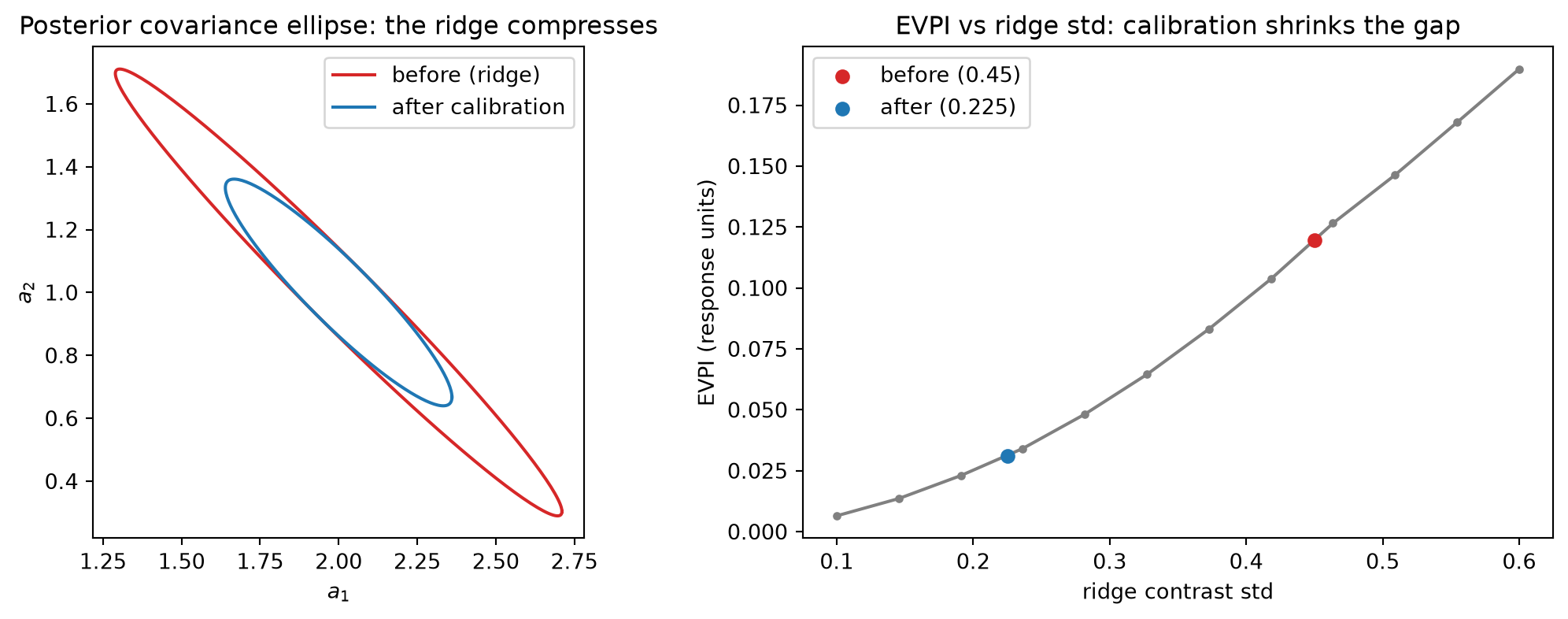
Reuse the Chapter 18 WE3 setup: a joint posterior on the channel coefficient vector a = (a_1, a_2) centered at (2, 1). The observational data pin the total-response direction (1,1)/\sqrt{2} tightly — the sales series identifies the overall level of spend response — while the attribution contrast direction u = (1,-1)/\sqrt{2} has posterior standard deviation 0.45, the ridge. This wide contrast posterior propagates through the equal-marginal optimizer (b_i^\star \propto a_i^2, from Chapter 18’s closed-form) into a wide distribution of optimal allocations: the posterior over b_1^\star spans combinations the business would treat as materially different decisions, and the resulting Chapter 18 EVPI is approximately 0.12 response units — the maximum a decision-maker should pay for an experiment that resolves the attribution contrast before committing to an allocation.
A geo lift experiment is now designed to measure the attribution split: it randomizes spend between the two channels across geographic markets, identifying which channel’s response drives the observed revenue lift. This estimand is a calibration factor on the contrast direction c = u = (1,-1)/\sqrt{2}, aimed precisely at the ridge. Applying the Rung 2 rank-one update with a calibration measurement precise enough to halve the contrast standard deviation — moving \sigma_{\text{contrast}} from 0.45 to 0.225, a fourfold increase in precision along u — the posterior in the ridge direction tightens by a factor of 4 in variance.
Propagating this tighter posterior through the Chapter 18 optimizer: the distribution of draw-specific optimal allocations b_1^\star(a^{(s)}) = B\,a_1^{(s)2}/(a_1^{(s)2}+a_2^{(s)2}) narrows in direct proportion to the tightening of the contrast draws. The EVPI, which scales approximately with the variance in the optimal-allocation distribution and hence with the variance in the attribution contrast, falls from approximately 0.12 to approximately 0.03 — a reduction of roughly 4\times, tracking the fourfold variance compression from the calibration. This is the wound of Chapter 18 closing. The wound was structural: observational MMM cannot identify the attribution contrast because the spend variation in the historical series was never designed to excite it independently. The calibration experiment bought back that identification. The EVPI gap, the maximum value of that identification expressed as a response-unit opportunity cost, shrinks from 0.12 to 0.03.