Theory & Proofs
The theory climbs a ladder, each rung resting on the one below. We begin with the smooth nonlinear program and its KKT conditions — the equations every method here is built to satisfy — then take the root-finding view that reads those conditions as a system of nonlinear equations. From there we develop Newton’s method and its quadratic convergence, prove the SQP keystone that each Newton step is itself a quadratic-programming subproblem, and replace the exact Hessian with the quasi-Newton (BFGS) update that makes the iteration practical. The upper rungs open the SLSQP internals — the least-squares recast, the active-set machinery, the merit-function line search — before confronting the non-convex reality of S-shaped response and closing on the real budget optimization. This part of the chapter builds the first rung: the program itself, and the first-order conditions that pin down its optima.
Rung 1 — The smooth program and its KKT conditions
Every method in this chapter is, at bottom, a machine for solving one system of equations — the KKT conditions of the program we are optimizing. Before we can iterate toward them we must state them precisely and earn the right to do so, for a general smooth program that need not be convex. Chapter 12 proved these conditions sufficient for a convex program: any KKT point there is the global optimum. Here we travel the other direction and establish them as the necessary conditions that every local minimizer of a smooth program must satisfy — the equations a solver is entitled to chase precisely because the optimum is guaranteed to lie among their solutions. We state the conditions in full and prove their first-order core.
The program. The general smooth nonlinear program is
\min_x\ f(x) \quad \text{subject to} \quad c_i(x) = 0\ (i \in \mathcal{E}), \qquad c_i(x) \le 0\ (i \in \mathcal{I}),
with the objective f and every constraint c_i twice continuously differentiable. The index sets \mathcal{E} and \mathcal{I} collect the equality and inequality constraints respectively. The device that couples objective to constraints is the Lagrangian, which attaches a scalar multiplier \lambda_i to each constraint and folds the program into a single function:
\mathcal{L}(x, \lambda) = f(x) + \sum_i \lambda_i c_i(x).
Active set and LICQ. At a feasible point x^\star the inequality constraints split into those touching the boundary and those with room to spare. The active set collects every equality together with the inequalities that hold with equality,
\mathcal{A}(x^\star) = \mathcal{E} \cup \{\, i \in \mathcal{I} : c_i(x^\star) = 0 \,\}.
Only active constraints can exert force at x^\star; an inactive inequality has strict slack and is locally irrelevant. For the multipliers to be well-defined the active gradients must not be degenerate, and the standard guarantee is a constraint qualification. The linear independence constraint qualification (LICQ) holds at x^\star when the active constraint gradients \{\nabla c_i(x^\star) : i \in \mathcal{A}(x^\star)\} are linearly independent. LICQ is what makes the tangent geometry of the feasible set faithful to its linearization — the hypothesis the proof below leans on directly.
Theorem (first-order necessary conditions / KKT). Suppose x^\star is a local minimizer of the program at which LICQ holds. Then there exist multipliers \lambda^\star such that
\nabla_x \mathcal{L}(x^\star, \lambda^\star) = \nabla f(x^\star) + \sum_i \lambda_i^\star \nabla c_i(x^\star) = 0 \quad\text{(stationarity)},
together with primal feasibility (c_i(x^\star) = 0 for i \in \mathcal{E} and c_i(x^\star) \le 0 for i \in \mathcal{I}), dual feasibility (\lambda_i^\star \ge 0 for i \in \mathcal{I}), and complementary slackness (\lambda_i^\star c_i(x^\star) = 0 for all i).
Proof (of the equality-constrained core). We prove the equality-only case — \min f(x) subject to c_i(x) = 0 for i \in \mathcal{E} — which carries the essential geometry; the inequality extension is stated immediately after and proved in full by Nocedal and Wright (2006).
Let x^\star be a local minimizer at which LICQ holds, and call a direction d a tangent direction if it is annihilated by every active constraint gradient,
\nabla c_i(x^\star)^\top d = 0 \quad \text{for all } i \in \mathcal{E}.
By LICQ the active Jacobian has full row rank, so the implicit function theorem furnishes a smooth feasible curve x(t) threading the constraint surface with
x(0) = x^\star, \qquad x'(0) = d, \qquad c_i(x(t)) = 0 \ \text{ for all } i \in \mathcal{E} \text{ and all } t \text{ near } 0.
The curve stays feasible by construction, so its objective value \phi(t) = f(x(t)) is a one-dimensional slice of f along the feasible set. Because x^\star is a local minimizer, t = 0 minimizes \phi, and a differentiable function at an interior minimum has vanishing derivative:
\phi'(0) = \nabla f(x^\star)^\top x'(0) = \nabla f(x^\star)^\top d = 0.
This holds for every tangent direction d. So \nabla f(x^\star) is orthogonal to the entire null space of the active Jacobian — equivalently, it lies in the orthogonal complement of that null space, which is the row space spanned by the active gradients \{\nabla c_i(x^\star)\}_{i \in \mathcal{E}}. Membership in that span means there exist scalars \lambda_i^\star with
\nabla f(x^\star) = -\sum_{i \in \mathcal{E}} \lambda_i^\star \nabla c_i(x^\star),
which rearranges to the stationarity condition \nabla_x \mathcal{L}(x^\star, \lambda^\star) = 0. \blacksquare
Inequality extension (stated). For inequality constraints the same argument restricted to the active set yields stationarity, and a first-variation argument over the cone of feasible directions forces the active multipliers to be nonnegative (\lambda_i^\star \ge 0): a binding constraint may only be approached from the feasible side, so its multiplier can push back in just one direction. Inactive constraints carry zero multiplier, which is exactly complementary slackness (\lambda_i^\star c_i(x^\star) = 0). The full proof is in Nocedal and Wright (2006). The sign condition is what distinguishes a binding constraint that pushes back on the optimum from one that is merely slack and exerts no force at all.
Second-order sufficient condition (stated). The KKT conditions are first-order: they locate stationary points but cannot by themselves separate a minimizer from a saddle. The curvature test that does is the second-order sufficient condition. If, in addition to KKT, the reduced Hessian of the Lagrangian is positive definite on the critical cone — d^\top \nabla^2_{xx} \mathcal{L}(x^\star, \lambda^\star)\, d > 0 for every nonzero d tangent to the active constraints — then x^\star is a strict local minimizer. This is the constrained analogue of the positive-definite-Hessian test from Chapter 12, restricted to the directions the active constraints leave free.
Tie to Chapter 12. There the KKT conditions were proved sufficient for convex programs: any KKT point is automatically a global optimum, because convexity makes stationarity certify optimality across the whole feasible set. Here they are the necessary conditions for a smooth, possibly non-convex program — the equations every solver in this chapter is built to satisfy, derived without any convexity assumption. For a convex problem the two readings coincide and KKT pins down the global optimum. For a non-convex one, KKT pins down only local optima, and a program may have many; that gap is exactly what the multi-start strategy later in the chapter is built to confront.
Rung 2 — The root-finding view
Rung 1 left us with a list of conditions a minimizer must satisfy: stationarity of the Lagrangian, plus feasibility. The decisive move of this chapter is to stop reading that list as a checklist and start reading it as a system of equations. Stationarity and feasibility, taken together, are simultaneous equations in the unknowns — and once we see them that way, the entire apparatus of nonlinear-equation solving, Newton’s method first among it, becomes available. That reframing is what this rung performs.
A KKT point is a root of a nonlinear system. Take the equality-constrained program and stack its two defining conditions into a single vector-valued map of the unknowns (x, \lambda):
F(x, \lambda) = \begin{bmatrix} \nabla f(x) + \nabla c(x)^\top \lambda \\ c(x) \end{bmatrix} = 0,
where c(x) is the vector of equality constraints and \nabla c(x) is their Jacobian, the matrix whose rows are the constraint gradients \nabla c_i(x)^\top. The top block is exactly stationarity, \nabla_x \mathcal{L} = 0; the bottom block is primal feasibility, c(x) = 0. A point (x^\star, \lambda^\star) satisfies the KKT conditions if and only if it is a root of F.
Solving the program is finding a root of F. This is the equivalence the rung is built on. The primal variables x and the multipliers \lambda are solved for together, as one coupled system: the multipliers are not an afterthought computed once x is known, but unknowns standing on equal footing with the decision variables, with their own block of equations (feasibility) and their own contribution to stationarity. The system F has as many equations as unknowns — n stationarity equations and m feasibility equations for n variables and m multipliers — so it is square, exactly the setting a root-finder requires.
Folding in inequalities. The construction above is written for equalities, but inequalities are absorbed with the active-set idea of Rung 1. At a solution, the active inequalities hold with equality and the inactive ones carry zero multiplier and can be dropped; treating the active inequalities as equalities inside F recovers a square system of precisely the form above. Which inequalities belong to the active set is itself a question — the active-set machinery that answers it is developed in the SLSQP rung. For the development of Newton’s method and SQP that follows, we take the active set as given, so F is square and smooth.
The pivot of the chapter. This single reframing — from “minimize f” to “solve F(x, \lambda) = 0” — is the hinge on which everything turns. Every method from here forward is a consequence of applying a nonlinear-equation solver to F: Newton’s method on F is the next rung, the SQP keystone shows each Newton step is a quadratic program, and SLSQP is the production solver for that iteration. We have stopped optimizing and started root-finding; the rest of the chapter cashes out that move.
Rung 3 — Newton’s method and quadratic convergence
We now have a square nonlinear system F(z) = 0 to solve, with z = (x, \lambda). The canonical solver for such a system is Newton’s method, and its defining virtue is quadratic convergence: once the iterate is close to a root, the error squares at every step. This is the property that makes SQP and SLSQP reach high accuracy in only a handful of iterations near the optimum — and it is a result the book has invoked but never proved. This rung supplies the proof.
Newton’s method for F(z) = 0. The idea is to replace F by its linear model at the current iterate and solve that exactly. Linearizing about z_k gives F(z_k + \Delta) \approx F(z_k) + F'(z_k)\Delta; setting the model to zero and solving for the step yields
F'(z_k)\, \Delta_k = -F(z_k), \qquad z_{k+1} = z_k + \Delta_k = z_k - F'(z_k)^{-1} F(z_k),
where F'(z_k) is the Jacobian of F at z_k. For the KKT system this Jacobian is the KKT matrix — the block matrix of Lagrangian-Hessian and constraint-Jacobian pieces that we assemble explicitly in the next rung; flag it here as the object every Newton step must factor.
Theorem (local quadratic convergence). Let F be C^2 with a root z^\star, F(z^\star) = 0, at which the Jacobian F'(z^\star) is nonsingular. Then there is a neighborhood of z^\star such that, started anywhere in it, Newton’s iterates converge to z^\star and satisfy
\|z_{k+1} - z^\star\| \le C\, \|z_k - z^\star\|^2
for a constant C — the error squares at each step.
Proof. Let e_k = z_k - z^\star denote the error at step k.
From the Newton update, subtract z^\star and insert F'(z_k)^{-1} F'(z_k) on the leading term:
\begin{aligned}
z_{k+1} - z^\star &= e_k - F'(z_k)^{-1} F(z_k) \\
&= F'(z_k)^{-1}\big[F'(z_k)\, e_k - F(z_k)\big].
\end{aligned}
Now Taylor-expand F around z_k and evaluate at z^\star, using F(z^\star) = 0:
\begin{aligned}
0 = F(z^\star) &= F(z_k) + F'(z_k)(z^\star - z_k) + R_k \\
&= F(z_k) - F'(z_k)\, e_k + R_k,
\end{aligned}
where the remainder is controlled by the C^2 assumption: \|R_k\| \le \tfrac12 L \|e_k\|^2, with L a Lipschitz constant for F' near z^\star. Rearranging the second display gives F'(z_k)\, e_k - F(z_k) = R_k, exactly the bracket in the first display, so
e_{k+1} = F'(z_k)^{-1} R_k, \qquad
\|e_{k+1}\| \le \|F'(z_k)^{-1}\|\, \|R_k\| \le \tfrac12 L\, \|F'(z_k)^{-1}\|\, \|e_k\|^2.
Finally, because F' is continuous and F'(z^\star) is nonsingular, \|F'(z_k)^{-1}\| \le 2\|F'(z^\star)^{-1}\| for every z_k close enough to z^\star. Substituting,
\|e_{k+1}\| \le C\, \|e_k\|^2, \qquad C = L\,\|F'(z^\star)^{-1}\|.
Shrinking the neighborhood so that C\|e_0\| < 1 forces the errors to contract — each step squares a quantity already below 1 — so z_k \to z^\star, and the squaring bound holds throughout. \blacksquare
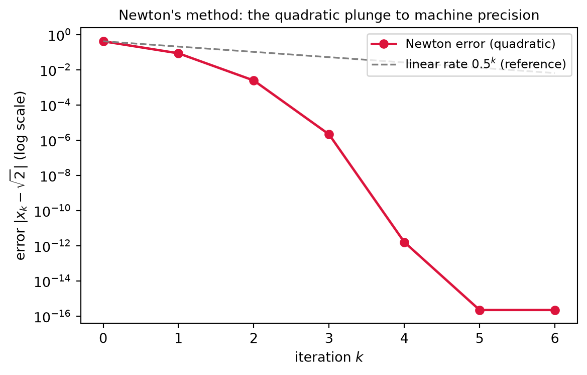
Digit-doubling. Quadratic convergence has a vivid reading: the number of correct digits roughly doubles at each step. If \|e_k\| \approx 10^{-3} then \|e_{k+1}\| \lesssim 10^{-6}, then 10^{-12} — three correct digits become six become twelve in two iterations. This is precisely why SQP and SLSQP attain high accuracy in only a handful of steps once they are near the solution; Worked Example 3 exhibits the squaring concretely on a scalar root, where the error column visibly halves its exponent’s distance to machine precision at every line.
The cost, and quasi-Newton. The rate is not free. Each Newton step needs the Jacobian F'(z_k), and for the KKT system that means second derivatives — the Hessian of f and of every constraint, assembled into the Lagrangian Hessian inside the KKT matrix. When those second derivatives are unavailable or too expensive, a quasi-Newton method approximates the Jacobian from first-derivative information accumulated across iterations, trading the quadratic rate for superlinear convergence — slower than quadratic, but still decisively faster than the linear rate of plain gradient methods. That construction is the BFGS update of Rung 5 (Nocedal and Wright 2006). Newton’s quadratic convergence is assumed nowhere earlier in this book; this rung supplies the proof, and it is exactly the engine that the SQP keystone of the next rung rides on.
Rung 4 — The keystone: SQP is Newton on the KKT system
This is the rung the chapter — and much of Part IV — has been climbing toward. Chapter 12 promised that SLSQP is “a Newton iteration on the KKT equations” that, at each step, “forms a quadratic model of the Lagrangian and a linearization of the constraints, solves that quadratic program for a search direction, and repeats.” Chapter 13 echoed it from the other side: the smooth, possibly non-concave world is the domain of an SLSQP that “attacks the nonlinear KKT system directly and iteratively.” Those were promissory notes. This rung pays them in full, and it does so by proving a single, surprising identity: the Newton step on the KKT system of Rung 2 is the solution of a quadratic-programming subproblem. The “quadratic model of the Lagrangian under a linearization of the constraints” is not a heuristic resemblance to Newton’s method — it is Newton’s method, written in another basis.
The KKT matrix and the Newton step
Rung 3 flagged that the Jacobian F'(z_k) of the root-finding map is the KKT matrix; we now assemble it explicitly. Differentiating the map F(x, \lambda) = \begin{bmatrix} \nabla f(x) + \nabla c(x)^\top \lambda \\ c(x) \end{bmatrix} from Rung 2 block by block gives
F'(x, \lambda) = \begin{bmatrix} \nabla^2_{xx}\mathcal{L}(x, \lambda) & \nabla c(x)^\top \\ \nabla c(x) & 0 \end{bmatrix}.
The top-left block follows from \partial_x[\nabla f + \nabla c^\top \lambda] = \nabla^2 f + \sum_i \lambda_i \nabla^2 c_i = \nabla^2_{xx}\mathcal{L} — the Hessian of the Lagrangian, not of f alone, because differentiating the multiplier-weighted constraint gradients pulls in the constraint curvatures \nabla^2 c_i. The top-right block is \partial_\lambda[\nabla f + \nabla c^\top \lambda] = \nabla c^\top. The bottom row differentiates the feasibility block c(x), giving the Jacobian \nabla c in the bottom-left and nothing in \lambda, hence the zero block. This symmetric, saddle-structured matrix is the object every Newton step must factor.
The Newton step (p, \delta\lambda) at the current iterate (x_k, \lambda_k) solves F'(x_k, \lambda_k)\begin{bmatrix} p \\ \delta\lambda \end{bmatrix} = -F(x_k, \lambda_k), which written out is
\begin{bmatrix} \nabla^2_{xx}\mathcal{L}_k & \nabla c_k^\top \\ \nabla c_k & 0 \end{bmatrix}\begin{bmatrix} p \\ \delta\lambda \end{bmatrix} = -\begin{bmatrix} \nabla f_k + \nabla c_k^\top \lambda_k \\ c_k \end{bmatrix},
with the subscript k marking evaluation at (x_k, \lambda_k). The step p updates the primal variable, x_{k+1} = x_k + p, and \delta\lambda updates the multiplier, \lambda_{k+1} = \lambda_k + \delta\lambda.
One change of variable cleans this up decisively. Solve for the new multiplier \lambda_{k+1} = \lambda_k + \delta\lambda rather than the increment. The top row currently reads \nabla^2_{xx}\mathcal{L}_k\, p + \nabla c_k^\top \delta\lambda = -\nabla f_k - \nabla c_k^\top \lambda_k; substituting \delta\lambda = \lambda_{k+1} - \lambda_k moves \nabla c_k^\top \lambda_k across to cancel the identical term on the right, leaving \nabla^2_{xx}\mathcal{L}_k\, p + \nabla c_k^\top \lambda_{k+1} = -\nabla f_k. The bottom row is unchanged. In the new multiplier the Newton block system is therefore
\begin{bmatrix} \nabla^2_{xx}\mathcal{L}_k & \nabla c_k^\top \\ \nabla c_k & 0 \end{bmatrix}\begin{bmatrix} p \\ \lambda_{k+1} \end{bmatrix} = -\begin{bmatrix} \nabla f_k \\ c_k \end{bmatrix}.
The right-hand side has shed the \lambda_k-dependent term entirely: it is now just the objective gradient and the constraint residual. This is the form we will recognize.
The theorem and proof
Theorem (SQP = Newton on KKT). The Newton step (p, \lambda_{k+1}) for the KKT system, as displayed above, is identical to the primal–dual solution of the quadratic-programming (QP) subproblem
\min_p\ \nabla f_k^\top p + \tfrac12 p^\top \nabla^2_{xx}\mathcal{L}_k\, p \quad\text{subject to}\quad \nabla c_k\, p + c_k = 0.
Each Newton iteration on the KKT conditions thus minimizes a quadratic model of the Lagrangian subject to a linearization of the constraints.
Proof. The strategy is to write down the KKT conditions of the QP subproblem itself and observe that they are the Newton block system verbatim. The QP is a constrained optimization problem in the step variable p, so it has its own first-order conditions — and by Rung 1 those conditions are exact and sufficient here, because the QP has a quadratic objective and linear constraints, so its feasible set is an affine subspace on which LICQ is the full-rank condition on \nabla c_k.
Introduce a multiplier \mu for the QP’s equality constraint \nabla c_k\, p + c_k = 0. The QP’s Lagrangian, in its own variables (p, \mu), is
\ell(p, \mu) = \nabla f_k^\top p + \tfrac12 p^\top \nabla^2_{xx}\mathcal{L}_k\, p + \mu^\top(\nabla c_k\, p + c_k).
Stationarity of the QP in p — differentiating \ell with respect to p and setting it to zero — gives
\nabla_p \ell = \nabla f_k + \nabla^2_{xx}\mathcal{L}_k\, p + \nabla c_k^\top \mu = 0, \qquad\text{i.e.}\qquad \nabla^2_{xx}\mathcal{L}_k\, p + \nabla c_k^\top \mu = -\nabla f_k.
Primal feasibility of the QP is the constraint itself,
\nabla c_k\, p + c_k = 0, \qquad\text{i.e.}\qquad \nabla c_k\, p = -c_k.
Stack these two conditions as a single block system:
\begin{aligned}
\begin{bmatrix} \nabla^2_{xx}\mathcal{L}_k & \nabla c_k^\top \\ \nabla c_k & 0 \end{bmatrix}\begin{bmatrix} p \\ \mu \end{bmatrix} = -\begin{bmatrix} \nabla f_k \\ c_k \end{bmatrix}.
\end{aligned}
This is exactly the Newton block system derived above, with the QP multiplier \mu occupying the slot of the updated multiplier \lambda_{k+1}. The two linear systems have the same matrix and the same right-hand side, so they have the same solution: the QP’s primal–dual optimizer (p, \mu) coincides with the Newton step (p, \lambda_{k+1}). Identifying \mu = \lambda_{k+1}, the Newton step on the KKT system is the solution of the QP subproblem. \blacksquare
After the proof
What it means. SQP is now fully named. Sequential Quadratic Programming is the algorithm that, at each iterate (x_k, \lambda_k), builds the QP subproblem above — a quadratic model of the Lagrangian, the term \tfrac12 p^\top \nabla^2_{xx}\mathcal{L}_k\, p together with the linear part \nabla f_k^\top p, minimized under a linearization of the constraints, \nabla c_k\, p + c_k = 0 — solves that QP for the step p and the new multipliers, updates x_{k+1} = x_k + p and \lambda_{k+1} = \mu, and repeats. The name is now literal: a sequence of quadratic programs. And because the theorem identifies each such QP solve with a Newton step on the KKT system, SQP inherits, untouched, the quadratic convergence proved in Rung 3 — near the solution the error squares at every iteration, and the digit-doubling of Rung 3 is the digit-doubling of SQP.
Why the Lagrangian, not just f. The single most important subtlety in the construction is that the quadratic model uses the Hessian of the Lagrangian \nabla^2_{xx}\mathcal{L}_k = \nabla^2 f_k + \sum_i (\lambda_k)_i \nabla^2 c_i(x_k), not the Hessian of the objective f alone. The constraints’ own curvature enters through the term \sum_i (\lambda_k)_i \nabla^2 c_i, weighted by the current multipliers. This is not optional polish. A method that modeled only \nabla^2 f would be building the wrong quadratic: it would ignore how the constraint surfaces bend away from their tangent linearization, and it would no longer be Newton’s method on the true KKT map F — the \nabla^2 c_i terms are precisely what differentiating \nabla c^\top \lambda produced when we assembled the KKT matrix. Modeling the Lagrangian is what makes the QP a genuine second-order model of the constrained problem rather than of the objective in isolation. The exception is illuminating: when every constraint is linear, \nabla^2 c_i = 0 and \nabla^2_{xx}\mathcal{L} = \nabla^2 f, so the distinction collapses — which is exactly the affine world of Chapter 13, where the constraint linearization \nabla c_k\, p + c_k = 0 is not an approximation at all but the constraint reproduced exactly.
Inequalities. The theorem above is stated for equality constraints, which carry the essential geometry. With inequality constraints the QP subproblem gains linearized inequalities \nabla c_i(x_k)^\top p + c_i(x_k) \le 0 for i \in \mathcal{I} alongside the linearized equalities. Solving that inequality-constrained QP requires deciding which linearized inequalities are active — the active-set computation, which is the machinery the SLSQP rung develops in detail (Nocedal and Wright 2006). But the heart of SQP is the equality result proved here: once the active set is fixed, the inequality QP reduces to an equality QP of exactly the form above, and the active-set logic is the orchestration around that core, not a replacement for it.
The redemption. State it plainly, because the whole part has been waiting for it. This is the result Chapter 12 named when it called SLSQP “a Newton iteration on the KKT equations” that “forms a quadratic model of the Lagrangian and a linearization of the constraints,” and the result Chapter 13 pointed to when it sent the smooth, non-concave world on to a solver that “attacks the nonlinear KKT system directly and iteratively.” Those phrases are no longer descriptions or promises. They are this theorem. SQP is Newton on the KKT system, the Newton step is a quadratic program, and the quadratic program is a model of the Lagrangian under a linearization of the constraints — one identity, proved. The keystone is set, and every rung above it now has something to rest on.
Rung 5 — The quasi-Newton Hessian
The keystone of Rung 4 hands us a clean algorithm — solve a QP at each iterate — but it hides a demand that, taken literally, would sink the method in practice: every QP subproblem needs the Lagrangian Hessian \nabla^2_{xx}\mathcal{L}_k for its quadratic term. Forming that matrix exactly is both expensive and, away from a solution, structurally dangerous. This rung confronts both problems and resolves them with a single device — a quasi-Newton (BFGS) approximation B_k that is built from first derivatives alone and is positive definite by construction. It is the modification that turns the elegant SQP iteration into something a solver can actually run.
Two problems with the exact Hessian. The quadratic model of Rung 4 calls for \nabla^2_{xx}\mathcal{L}_k = \nabla^2 f_k + \sum_i (\lambda_k)_i \nabla^2 c_i(x_k), and that object resists use on two fronts. (i) Cost. It requires the second derivatives of the objective and of every constraint — a full Hessian for f and one for each c_i, assembled and weighted by the current multipliers. For real problems those second derivatives are frequently unavailable in closed form or far too expensive to compute and store at every iteration. (ii) Indefiniteness. Even when the exact Hessian is in hand, away from a solution \nabla^2_{xx}\mathcal{L}_k may be indefinite — it carries directions of negative curvature. A QP whose quadratic term is indefinite is nonconvex: it has no unique minimizer, and on the linearized feasible set its objective may be unbounded below, so the QP solver has nothing well-defined to return. The subproblem the keystone hands us is only as useful as the QP solver’s ability to minimize it, and that solver needs a convex model.
The BFGS approximation. Both problems dissolve if we never form the exact Hessian at all and instead maintain a symmetric positive-definite matrix B_k \approx \nabla^2_{xx}\mathcal{L}_k, updated from the first-derivative information the iteration already produces. Across a step we observe two vectors — how far the iterate moved, and how the Lagrangian’s gradient changed over that move:
s_k = x_{k+1} - x_k, \qquad y_k = \nabla_x \mathcal{L}(x_{k+1}, \lambda_{k+1}) - \nabla_x \mathcal{L}(x_k, \lambda_{k+1}).
Both gradients are taken at the same multiplier \lambda_{k+1}, so y_k isolates the change in curvature of the Lagrangian in x alone. The BFGS update folds this observed curvature into the next approximation,
B_{k+1} = B_k - \frac{B_k s_k s_k^\top B_k}{s_k^\top B_k s_k} + \frac{y_k y_k^\top}{y_k^\top s_k}.
It is the rank-two update — two symmetric rank-one corrections, one subtracted and one added — that satisfies the secant equation
B_{k+1} s_k = y_k
while keeping B_{k+1} symmetric. The secant equation is the demand that the new approximation reproduce the observed curvature along s_k: applied to the step just taken, B_{k+1} returns exactly the gradient change that step produced. This is the finite-difference analogue of the defining Hessian relation, and it is the sense in which B_k accumulates true second-order information from a trail of first-order evaluations.
Curvature condition and Powell damping. The construction’s prize is that positive definiteness propagates: if B_k \succ 0, then B_{k+1} \succ 0 — provided the curvature condition
s_k^\top y_k > 0
holds, which keeps the added rank-one term y_k y_k^\top / (y_k^\top s_k) well-defined and positive. For a convex problem the curvature condition is automatic, but on a nonconvex problem it can fail — s_k^\top y_k may be zero or negative, and a raw BFGS update would then destroy definiteness. Powell’s damping repairs this by replacing y_k with a convex combination of y_k and B_k s_k,
\hat y_k = \theta y_k + (1 - \theta) B_k s_k, \qquad \theta \in (0, 1],
with \theta chosen as large as possible subject to s_k^\top \hat y_k \ge 0.2\, s_k^\top B_k s_k. Because B_k \succ 0 makes s_k^\top B_k s_k > 0, the damped vector always satisfies s_k^\top \hat y_k > 0, so updating with \hat y_k in place of y_k guarantees B_{k+1} \succ 0 unconditionally. The payoff is exactly the property the QP solver demanded: with B_k \succ 0 in the quadratic term, every QP subproblem is a convex QP, with a unique, well-defined minimizer.
Convergence and a key consequence. Substituting B_k for the exact Hessian is not free: with an approximate Jacobian the iteration is no longer pure Newton, so the exact quadratic convergence of Rung 3 is lost. What survives is superlinear convergence — slower than quadratic, but still decisively faster than the linear rate of gradient methods, and fast enough that the digit count climbs sharply near the solution (Nocedal and Wright 2006). There is a second consequence that matters even more for what follows. Because B_k \succ 0, the step p returned by the convex QP is a descent direction for a merit function that balances objective and constraint violation — moving along p decreases that merit. This is the hook that the line search of Rung 6 will grip when it globalizes the method: positive definiteness of B_k is precisely what guarantees there is something to descend along. Flag it now; the next rung collects on it.
Rung 6 — Inside SLSQP
With the BFGS Hessian in place we have a complete conceptual algorithm; this rung opens the three engineering pieces that turn that algorithm into the production solver SLSQP — a numerically stable least-squares solve of each QP subproblem (part a), an active-set strategy that decides which inequalities bind (part b), and a merit-function line search that delivers global convergence (part c). We develop the least-squares recast here and take up the active set and the line search next.
(a) The least-squares recast
The positive definiteness won in Rung 5 is not merely a convexity guarantee — it is the structural fact that lets the QP be solved in its most numerically stable form. Because B_k \succ 0, it admits a Cholesky factorization (Chapter 1)
B_k = L_k L_k^\top,
with L_k lower-triangular and carrying a strictly positive diagonal. This factor is exactly what turns the QP’s quadratic objective into a perfect square plus a constant:
\tfrac12 p^\top B_k p + \nabla f_k^\top p = \tfrac12 \big\| L_k^\top p + L_k^{-1}\nabla f_k \big\|^2 - \tfrac12 \big\| L_k^{-1}\nabla f_k\big\|^2.
To see this, complete the square — expand the squared norm on the right and use L_k L_k^\top = B_k together with L_k L_k^{-1} = I:
\begin{aligned}
\tfrac12 \big\| L_k^\top p + L_k^{-1}\nabla f_k \big\|^2
&= \tfrac12 p^\top L_k L_k^\top p + p^\top L_k L_k^{-1}\nabla f_k + \tfrac12 \big\| L_k^{-1}\nabla f_k \big\|^2 \\
&= \tfrac12 p^\top B_k p + \nabla f_k^\top p + \tfrac12 \big\| L_k^{-1}\nabla f_k \big\|^2.
\end{aligned}
Subtracting the constant \tfrac12 \| L_k^{-1}\nabla f_k\|^2 from both sides returns the QP objective exactly, which is the identity displayed above.
Consequence. The constant term carries no p, so minimizing the QP objective is identical to minimizing the Euclidean norm \| L_k^\top p + L_k^{-1}\nabla f_k\| — a linear least-squares objective in the step p. Subject to the linearized constraints of Rung 4, the QP subproblem is therefore a linearly-constrained linear least-squares problem: a least-squares objective under the equality and inequality linearizations, the structure known in the numerical-optimization literature as LSEI (least squares with equality and inequality constraints), itself reducible to a nonnegative least squares (NNLS) problem.
Why this matters numerically. Casting the QP as least squares lets SLSQP solve each step with stable orthogonal (QR) factorizations and never form B_k^{-1} or factor the indefinite KKT matrix of Rung 4 directly. Working through the Cholesky factor L_k rather than the matrix B_k keeps the computation on the square root of the problem’s conditioning — the conditioning is never squared, as it would be by forming and factoring B_k or its inverse — and the positive definiteness of B_k is exploited structurally, as the very thing that makes the Cholesky factor exist. This is the “Sequential Least Squares” in the name SLSQP: each SQP step is solved as a constrained least-squares problem. The algorithm is Kraft’s (1988); its underlying theory is developed in full by Nocedal and Wright (2006).
(b) The active-set strategy
Part (a) showed how to solve a QP whose constraints are all equalities — the least-squares form. But the QP subproblem of Rung 4 carries linearized inequality constraints \nabla c_i(x_k)^\top p + c_i(x_k) \le 0 for i \in \mathcal{I}, and an inequality-constrained QP must first decide which of them hold with equality at its solution before any equality-form solve can run. The active-set method makes that decision, and it makes it by repeatedly invoking part (a).
Working set. Maintain a working set \mathcal{W} of inequality constraints provisionally treated as equalities, sitting alongside the genuine equalities \mathcal{E}. With \mathcal{W} held fixed, every constraint in play is an equality, and the QP collapses to exactly the equality-constrained least-squares problem of part (a) — the one solvable form we possess. Solving it yields a candidate step p together with a multiplier for each working-set constraint. The whole strategy is a loop that guesses \mathcal{W}, solves the resulting equality QP, and then corrects the guess.
The two checks that update \mathcal{W}. After each equality-constrained solve, two tests decide whether the current working set is right, and if not, how to amend it:
- Drop a constraint. If a working-set inequality has a negative multiplier, KKT dual feasibility (\lambda_i \ge 0) is violated: that constraint is “pulling the wrong way,” holding the step back against the objective rather than truly binding. Removing it from \mathcal{W} and re-solving lowers the objective. Drop the constraint with the most negative multiplier.
- Add a constraint. If a constraint outside \mathcal{W} is violated by the candidate step — its linearized inequality would be exceeded — then p is infeasible and must be reined in. Add that constraint to \mathcal{W}, typically via a ratio test that finds the first constraint hit as one moves along p, and re-solve.
- Termination of the inner loop. Iterate until no working-set multiplier is negative and no outside constraint is violated. At that point the working set is consistent with the QP’s KKT conditions: every constraint in \mathcal{W} binds with a nonnegative multiplier, every constraint outside is satisfied with slack, and the equality solve over \mathcal{W} is the QP’s true optimum.
This is complementary slackness, computed. The loop is complementary slackness enforced combinatorially. Recall from Chapter 12 that KKT optimality demands \lambda_i\, c_i = 0 for each inequality — each constraint is either active (binding, with multiplier \ge 0) or inactive (slack, with multiplier 0), never both. The active-set method does not assume that partition; it searches for it, dropping constraints whose multipliers turn negative and adding constraints that the step violates until the active/inactive split is self-consistent. This is precisely the logic Chapter 13’s simplex method used as it moved between LP vertices, each vertex a choice of which constraints are tight — here transplanted inside every QP subproblem of the nonlinear iteration. Because there are only finitely many possible working sets, the inner loop terminates (with the standard anti-cycling safeguards, exactly as in LP).
(c) The merit-function line search
The SQP step p inherits Newton’s bargain: the fast quadratic/superlinear convergence of Rungs 3 and 5 holds only near a solution. From a poor starting point the full step can increase the objective, or worsen the constraint violation, or both — the local model is simply not yet trustworthy. To globalize the method we need two things: a single scalar that measures progress when objective and feasibility may pull in opposite directions, and a rule for shortening the step when it overreaches. The merit function supplies the measure; the line search supplies the shortening.
The \ell_1 merit function. Fold the objective and the total constraint violation into one scalar,
\phi(x; \mu) = f(x) + \mu \Big( \sum_{i\in\mathcal{E}} |c_i(x)| + \sum_{i\in\mathcal{I}} \max\{0,\, c_i(x)\} \Big),
with penalty parameter \mu > 0. The second term is zero exactly at feasible points and grows with the amount of violation — equalities penalized by |c_i|, inequalities by their positive part \max\{0, c_i\}. Thus \phi is small only where f is small and the constraints are nearly satisfied, so a decrease in \phi is a single, honest measure of progress toward a KKT point — it cannot be fooled by an objective that drops only by fleeing feasibility.
The line search. Take a damped step x_{k+1} = x_k + \alpha_k p with \alpha_k \in (0, 1] chosen by backtracking: start at \alpha = 1 — the full SQP step, so that the fast local rate is preserved the moment it becomes available — and halve \alpha until \phi decreases sufficiently, an Armijo-type condition imposed on \phi rather than on f alone.
The descent property. Here Rung 5’s flag is collected. For \mu chosen large enough — in particular exceeding the largest multiplier magnitude, \mu > \|\lambda_{k+1}\|_\infty — the SQP direction p is a descent direction for \phi: the directional derivative satisfies
D_p\, \phi(x_k; \mu) < 0.
The reason joins the two halves of the construction. The QP step reduces the linearized model of f along p by an amount controlled by B_k, and because B_k \succ 0 (Rung 5) that reduction is a genuine decrease, not a numerical accident. At the same time the linearized constraints in the QP drive the linearized violation to zero along p. With \mu large enough, the guaranteed violation-reduction term dominates any first-order increase in the objective, so \phi strictly decreases for small \alpha. A satisfactory step length therefore always exists, which is exactly what backtracking finds — yielding global convergence to a KKT point from arbitrary starting points (the full proof is in Nocedal and Wright (2006)).
The Maratos effect. One subtlety: very near the solution the \ell_1 merit function can occasionally reject the full, well-converged step — forcing \alpha < 1 and stalling the fast local rate — even though that step is excellent; a second-order correction to the step repairs the pathology and restores the superlinear rate.
Synthesis. Assembling Rung 6 closes the algorithmic core of the chapter. SLSQP is damped-BFGS SQP — a convex quadratic model of the Lagrangian (Rungs 4–5) — plus the least-squares QP solve (part a), plus the active-set strategy (part b), plus the merit-function line search (part c). Local superlinear speed and global reliability, in one method. And this is no abstraction: it is precisely the algorithm invoked by scipy.optimize.minimize(method="SLSQP") — the solver a real budget optimizer runs.
Rung 7 — Local solutions and multi-start
Rung 6 ended on a strong word: global convergence. The merit-function line search drives SLSQP, from any starting point, to a point where the iteration stops moving — and that resting point satisfies the KKT conditions. It is tempting to read “global convergence” as “converges to the global optimum.” It does not. The adjective global describes the starting point, not the answer: convergence from anywhere to a KKT point. What that KKT point is worth depends entirely on the problem’s shape, and this rung draws the line precisely.
What is guaranteed. SLSQP converges, from an arbitrary initial allocation, to a point x^\star satisfying the KKT conditions of Rung 1 — stationarity of the Lagrangian, primal and dual feasibility, complementary slackness. By the first-order theory this certifies x^\star as a local optimum and a stationary point of the Lagrangian. That is a real guarantee, and it is the most any smooth local method can promise.
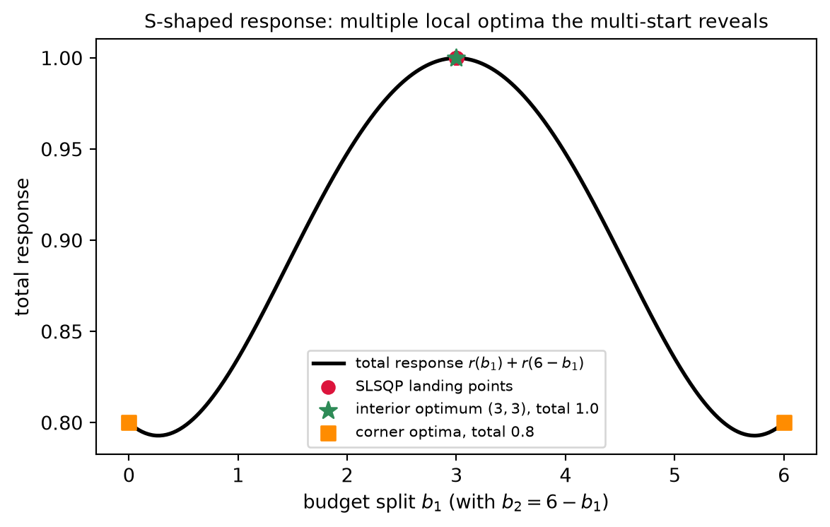
What is not. A local KKT point is the global optimum only if the problem is convex — convex objective over a convex feasible set. This is exactly Chapter 12’s keystone: every local minimum of a convex problem is global, and outside the convex world that implication simply fails. For a non-convex problem the failure is not hypothetical. An S-shaped response curve — the realistic media-saturation shape, with a convex toe at low spend before the concave saturation sets in — destroys concavity at the very bottom of its range, and a sum of such curves over a budget simplex generically presents several KKT points with different objective values: interior splits, corner allocations, mixtures. SLSQP from a single start finds exactly one of them, and which one is decided by the initialization — the algorithm slides downhill into whichever basin it began in and certifies the local optimum at the bottom. So the Rung 6 guarantee and the Chapter 12 keystone meet here at a single, often-confused distinction: convergence from anywhere to a KKT point is not convergence to the global optimum. The two coincide only when the problem is convex.
The remedy: multi-start. When the problem is non-convex and smooth, the practical answer is multi-start: run SLSQP from many initial allocations spread across the feasible set, let each converge to its local KKT point, and keep the best one found. The logic is simple — different starts fall into different basins, so a spread of starts samples a spread of local optima, and with enough well-placed starts one is likely to begin inside the basin of the global optimum and be carried there. But “likely” is the honest word: multi-start is a strategy, not a certificate. It returns the best optimum it happened to find, and nothing in it proves no better optimum exists elsewhere. This is precisely the boundary Chapters 12 and 13 drew and refused to blur — certainty lives in the convex world; outside it, we are diligent, not certain.
Genuinely global methods do exist — branch-and-bound exploits special structure to certify the global optimum, and Bayesian optimization and related global-search methods attack black-box problems without derivatives — but they are out of scope here; for the smooth non-convex budget problems of this book, multi-start SLSQP is the practical standard.
Rung 8 — The capstone: optimizing the real budget
Everything in Part IV has been climbing toward one problem. Chapter 12 built the convex theory and derived the equal-marginal rule by hand; Chapter 13 approximated the budget problem with a linear program and read the shadow price off the dual; this chapter built the production solver. Now they converge — on the smooth budget-allocation problem that the LP could only approximate and that SLSQP solves exactly.
(a) The concave case — vindication. Write the budget problem on a smooth concave response,
\max_{b\ge 0}\ \sum_i r_i(b_i) \quad\text{s.t.}\quad \mathbf{1}^\top b = B \quad (\text{+ per-channel caps}),
each r_i smooth and concave, which SLSQP solves in the standard minimization form \min\, -\sum_i r_i(b_i) under the same constraints. Because each -r_i is convex and the feasible set — a budget hyperplane intersected with box caps — is convex, the problem is convex, and by Rung 7 (Chapter 12’s keystone) the local KKT point SLSQP returns is the unique global optimum. The KKT stationarity it satisfies is nothing other than Chapter 12’s equal-marginal condition r_i'(b_i^\star) = \lambda across funded channels, and the Lagrange multiplier SLSQP returns on the budget constraint is exactly that \lambda — the shadow price of the budget, handed back by the solver for free.
Take the worked instance one last time: square-root response r_i(b) = a_i\sqrt{b}, coefficients a = (2, 1), budget B = 9. SLSQP converges to
b^\star = (7.2,\ 1.8), \qquad \lambda = 0.3727, \qquad \sum_i r_i(b_i^\star) = 6.7082,
identical to Chapter 12’s hand derivation from the equal-marginal condition and to Chapter 13’s refined-LP dual price — but now with no piecewise-linear approximation. Chapter 13 reached these numbers only in the limit, as its segmentation refined and the discretization error went to zero; SLSQP solves the smooth problem directly and lands on them at once. This is the convergence of the entire Part IV arc: convex theory (Ch 11), LP duality (Ch 12), and the SQP solver (Ch 13) arrive at the same allocation (7.2, 1.8) and the same shadow price \lambda = 0.3727 from three independent directions — the analytic, the linear-programming, and the iterative-Newton. Three methods, one answer; that is what vindication looks like.
(b) The S-shaped case — why we needed SLSQP. Replace the concave response with a Hill curve of exponent n > 1 — a convex toe rising into a concave shoulder. The sum of such curves over the budget simplex is non-concave, so the budget problem is non-convex, and Rung 7 applies in full: a single SLSQP run finds a local optimum that depends on its start, and multi-start is required to trust the result. The arithmetic makes the trap concrete. Two channels with Hill exponent n = 2 and half-saturation K = 3, budget B = 6. The interior split b = (3, 3) earns total response 1.0, while the corner allocations b = (6, 0) and b = (0, 6) earn only 0.8. All three are KKT points — each satisfies stationarity and the constraints — yet they are not equal in value, and an SLSQP run started near a corner converges to that inferior corner and certifies it, never seeing the better interior split. Multi-start, sweeping a spread of initial allocations, finds the superior interior optimum that the corner start misses. This is precisely the case Chapter 13’s “fill steepest first” heuristic got wrong — the convex toe means the steepest-first greedy ordering can pour the whole budget into one channel and miss the balanced split — and the case a single descent run cannot be trusted on. It is the case this chapter was built for. (The Code Tie-in runs the multi-start and exhibits both outcomes — the corner trap and the interior recovery — on exactly this Hill instance.)
Bridge to Part V. This closes the Theory section, and with it the optimization mathematics of Part IV — but the response curves r_i have so far been given. They will not be. A fitted MMM posterior, the work of Parts II–III, is what supplies the response curves: the saturation parameters are estimated, so each r_i comes with uncertainty, and the curves are themselves random — one draw of r_i per posterior draw. Chapter 18’s budget-optimization chapter runs this very solver against those fitted curves, typically once per posterior draw, to allocate spend under that uncertainty and propagate it into the optimal allocation. Part IV built the machinery from the ground up — convex foundations (Ch 11), linear programming (Ch 12), the production constrained solver (Ch 13); Part V turns it loose on a real, fitted model. The theory ends here.
Worked Examples
The three calculations with the most arithmetic — taking one SQP step by hand, solving the concave budget optimum exactly, and watching Newton’s error square line by line — are each small enough to carry out with pen and paper. Working them once turns the abstractions of the Theory section into numbers you can check: the KKT block system of Rung 4 becomes a 3\times3 solve, the budget capstone of Rung 8 becomes a two-line stationarity calculation, and the quadratic convergence of Rung 3 becomes a column of errors whose exponent doubles. The first example shows why SQP solves a quadratic-with-linear-constraint problem in a single step; the second shows the answer all of Part IV converges on; the third shows the speed that makes the whole method practical.
Example 1 — One SQP step on an equality-constrained problem
Take the smallest non-trivial constrained problem,
\min\ x_1^2 + x_2^2 \quad\text{subject to}\quad x_1 + x_2 = 2,
and run a single SQP step on it by hand. The objective is f = x_1^2 + x_2^2 with gradient \nabla f = (2x_1, 2x_2); the one equality is c(x) = x_1 + x_2 - 2 with gradient \nabla c = (1, 1). The Lagrangian \mathcal{L} = x_1^2 + x_2^2 + \lambda(x_1 + x_2 - 2) has Hessian
\nabla^2_{xx}\mathcal{L} = \begin{bmatrix} 2 & 0 \\ 0 & 2 \end{bmatrix} = 2I,
with the constraint contributing no curvature — it is linear, so \nabla^2 c = 0 and the Lagrangian Hessian is just \nabla^2 f (exactly the collapse Rung 4 flagged for linear constraints).
Assemble the block system. Start at x_0 = (0, 0) with \lambda_0 = 0. Then \nabla f_0 = (0, 0), the constraint residual is c_0 = 0 + 0 - 2 = -2, and \nabla c_0 = (1, 1). The Newton/SQP block system of Rung 4, \begin{bmatrix} \nabla^2_{xx}\mathcal{L} & \nabla c^\top \\ \nabla c & 0 \end{bmatrix}\begin{bmatrix} p \\ \lambda_1 \end{bmatrix} = -\begin{bmatrix} \nabla f_0 \\ c_0 \end{bmatrix}, is
\begin{bmatrix} 2 & 0 & 1 \\ 0 & 2 & 1 \\ 1 & 1 & 0 \end{bmatrix}\begin{bmatrix} p_1 \\ p_2 \\ \lambda_1 \end{bmatrix} = \begin{bmatrix} 0 \\ 0 \\ 2 \end{bmatrix},
where the right-hand side is -[\nabla f_0;\, c_0] = -[0, 0, -2] = [0, 0, 2].
Solve. Rows 1 and 2 read 2p_1 + \lambda_1 = 0 and 2p_2 + \lambda_1 = 0, so p_1 = p_2 = -\lambda_1/2. Substituting into row 3, p_1 + p_2 = 2, gives -\lambda_1 = 2, hence
\lambda_1 = -2, \qquad p_1 = p_2 = 1, \qquad p = (1, 1).
The step lands at x_1 = x_0 + p = (1, 1) with multiplier \lambda_1 = -2.
Interpretation. A single step reaches the exact optimum (1, 1), where f = 2. The reason is the keystone of Rung 4 read in reverse: the objective is quadratic and the constraint linear, so the QP subproblem SQP builds is identical to the original problem — its quadratic model of the objective is exact, not an approximation, and its linearized constraint \nabla c_0\, p + c_0 = 0 reproduces the true constraint x_1 + x_2 = 2 verbatim. One Newton/SQP step solves that QP outright, so it solves the original problem outright. With a nonlinear constraint the linearization would only be a local approximation and several steps would be needed, refreshing the linearization each time — that iteration is exactly what the Code Tie-in exhibits. We can confirm the answer independently: by symmetry the true optimum has x_1 = x_2 = 1, and the stationarity condition 2x_i + \lambda = 0 holds with \lambda = -2, matching the multiplier the step returned.
Example 2 — The concave budget optimum
This is the capstone instance of Rung 8, solved exactly by the KKT stationarity conditions. Maximize the total square-root response
\max_{b \ge 0}\ \sum_i a_i \sqrt{b_i} \quad\text{subject to}\quad b_1 + b_2 = 9,
with coefficients a = (2, 1). Each channel’s response r_i(b_i) = a_i\sqrt{b_i} is smooth and concave, so the problem is convex and the KKT point is the global optimum.
Equal-marginal condition. Stationarity is Chapter 12’s equal-marginal rule: at the optimum the marginal return r_i'(b_i) = \dfrac{a_i}{2\sqrt{b_i}} equals the common budget multiplier \lambda for every funded channel. Setting the two marginals equal,
\frac{a_1}{2\sqrt{b_1}} = \frac{a_2}{2\sqrt{b_2}} \quad\Longrightarrow\quad \frac{a_1^2}{b_1} = \frac{a_2^2}{b_2} \quad\Longrightarrow\quad \frac{b_1}{b_2} = \frac{a_1^2}{a_2^2} = \frac{4}{1} = 4.
Solve with the budget. With b_1 = 4 b_2 and b_1 + b_2 = 9,
4 b_2 + b_2 = 9 \quad\Longrightarrow\quad 5 b_2 = 9 \quad\Longrightarrow\quad b_2 = 1.8, \qquad b_1 = 7.2,
so the optimal allocation is b^\star = (7.2,\ 1.8).
The common multiplier. Evaluate the shared marginal return at the optimum,
\lambda = \frac{a_1}{2\sqrt{b_1}} = \frac{2}{2\sqrt{7.2}} = \frac{1}{\sqrt{7.2}} \approx 0.3727.
Total response. Summing the two channels,
2\sqrt{7.2} + \sqrt{1.8} = 2(2.6833) + 1.3416 = 6.7082.
Interpretation. This is the problem solved three ways, and all three agree. Chapter 12 derived (7.2, 1.8) with \lambda = 0.3727 from the equal-marginal condition by hand; Chapter 13 reached the same allocation as a refined-LP dual price, in the limit as its piecewise-linear segmentation grew fine; and SLSQP returns precisely this allocation and this multiplier on the budget constraint, solving the smooth problem directly with no piecewise-linear approximation at all. The Lagrange multiplier SLSQP hands back is \lambda, the shadow price of the budget. Three methods — analytic, linear-programming, and iterative-Newton — converging on one answer is the payoff of the entire Part IV arc.
Example 3 — Newton’s method squares the error
The quadratic convergence proved in Rung 3 is easiest to see on a scalar root. Solve g(x) = x^2 - 2 = 0 for \sqrt{2} by Newton’s method. The iteration x_{k+1} = x_k - \dfrac{g(x_k)}{g'(x_k)} becomes
x_{k+1} = x_k - \frac{x_k^2 - 2}{2 x_k} = \frac12\Big(x_k + \frac{2}{x_k}\Big),
the classical Babylonian square-root iteration. Starting from x_0 = 1, tabulate each iterate and its error against \sqrt{2} = 1.41421356\ldots:
| 0 |
1.000000000000 |
4.14\times10^{-1} |
| 1 |
1.500000000000 |
8.58\times10^{-2} |
| 2 |
1.416666666667 |
2.45\times10^{-3} |
| 3 |
1.414215686275 |
2.12\times10^{-6} |
| 4 |
1.414213562375 |
1.59\times10^{-12} |
Interpretation. Each error is roughly the square of the previous one, times a constant \approx \frac{1}{2\sqrt2} \approx 0.354. Reading down the error column, 8.6\times10^{-2} \to 2.5\times10^{-3} \to 2.1\times10^{-6} \to 1.6\times10^{-12}: the exponent roughly doubles at each step, which is the digit-doubling of Rung 3’s theorem made concrete. Three correct digits become six become twelve in just two iterations. This is exactly why SLSQP — which Rung 4 proved to be Newton’s method on the KKT system — needs only a handful of iterations to reach high accuracy once it is near the optimum: the same squaring that drives this scalar error to 10^{-12} in four steps drives the constrained iteration to its KKT point, and it is precisely the 7 iterations the Code Tie-in’s concave solve will take.