Chapter 23 grounded the computation an MMM performs — the arithmetic and its cost. This chapter grounds the structure that holds the computation together. A working marketing-mix system is not one program but many parts that change at different rates: data ingestion adapters churn as upstream sources shift, reporting is rewritten whenever stakeholders want a new view, while the response-curve abstraction and the prior store at the system’s heart should change almost never. The driving question is the architect’s: the MMM stack is many parts that evolve at different rates — how do you structure them so a component can be built, tested, and replaced without disturbing the rest, and so the calibration loop doesn’t tangle everything together?
The answer this chapter develops is a single structural property. Model the system as a graph whose nodes are modules and whose edges are dependencies; good architecture is the demand that this graph be acyclic, with dependencies pointing toward the parts that change least. The center of gravity is therefore a theorem about directed graphs — a dependency graph admits a buildable, testable ordering exactly when it has no cycles — and the supporting framework is Robert Martin’s Clean Architecture (Martin 2017): the instability metric that says which way dependencies should point, and the Dependency Rule that keeps them pointing that way.
The payoff that unifies the chapter concerns the Part VI calibration–optimization loop. At runtime that loop genuinely cycles: the optimizer flags a high-leverage spend region, an experiment is run there, calibration folds the result into the posterior, the store updates, and the optimizer runs again. It is tempting to conclude that the modules must therefore depend on each other in a cycle — and if they did, none of them could be built or tested alone. They need not. A runtime data cycle is not a source-code dependency cycle. Routing the optimizer and the calibration step through the stable prior-store interface, rather than letting them depend on each other, keeps the module graph acyclic while the data still flows around the loop. That move is exactly Clean Architecture’s Dependency Rule, and it is what makes the Part VI system maintainable rather than a tangle.
The modules used throughout are the ones the book has already built: a stable domain core — the response curve S(x;\theta) and the prior-store interface — together with ingestion, transforms (adstock and saturation), fit, store, calibration, optimizer, and reporting.
24.2 Theory & Proofs
The five rungs build from the unit to the whole system. Rung 1 fixes what a module is and how to measure coupling. Rung 2 puts the modules into a dependency graph and quantifies which are stable. Rung 3 is the keystone: the dependency graph is buildable and testable in pieces exactly when it is acyclic. Rung 4 resolves the apparent contradiction of the calibration loop, distinguishing data cycles from dependency cycles. Rung 5 assembles the layered MMM architecture and hands off to the rest of Part VII.
24.2.1 Rung 1 — Modules, interfaces, coupling, and cohesion
A module is a unit of software with a public interface that hides its internal decisions. The principle is information hiding (Parnas 1972): a module exposes what it does and conceals how, so that consumers depend only on the interface and the implementation is free to change behind it. The MMM’s fit module, for instance, exposes “given data and priors, return a posterior” and hides whether that posterior is computed by one sampler or another — a decision Chapter 23 showed is consequential but, properly hidden, local.
Two qualities govern a decomposition into modules. Cohesion is the relatedness of what lives inside a single module; it should be high, so that a module has one clear responsibility. Coupling is the dependence between modules; it should be low, so that changing one module forces few changes elsewhere. These are made countable by the dependency relation: the fan-out of a module is the number of modules it depends on, and its fan-in is the number of modules that depend on it. A module with high fan-in is relied upon by much of the system; a module with high fan-out relies on much of the system. The next rung turns these counts into a single measure of how safely a module can change.
24.2.2 Rung 2 — The dependency graph and the instability metric
Model the system as a directed graph G = (V, E) in which V is the set of modules and an edge u \to v means “u depends on v.” Martin’s instability of a module measures how exposed it is to change in others relative to how much others are exposed to change in it:
A module with I = 0 has only incoming edges: nothing it depends on can force it to change, while everything that depends on it constrains it — it is maximally stable. A module with I = 1 has only outgoing edges: it depends on others but nothing depends on it, so it is free to change at will — it is maximally unstable.
The Stable Dependencies Principle follows: dependencies should point in the direction of decreasing instability, from less stable modules toward more stable ones. The reason is asymmetric risk. If a volatile module depends on a stable one, changes in the volatile module are absorbed locally; but if a stable module depended on a volatile one, every churn in the volatile module would ripple into the part of the system everything else relies on. In the MMM graph the domain core has I = 0 — many modules depend on the response curve and the store interface, and the core depends on nothing — while reporting and ingestion sit at I = 1 as leaves that only consume. The prior store is deliberately kept stable, with high fan-in and low instability, because so much of the system is built on it.
24.2.3 Rung 3 — Acyclicity ⇔ a topological order exists (keystone)
A topological order of G is a linear arrangement of its modules in which every edge points forward — every module appears after all the modules it depends on. Such an order is precisely a valid build, initialization, and test sequence: each module is constructed using only modules already in place. The keystone of the chapter is that such an order exists exactly when the dependency graph has no cycles.
Theorem. A finite directed graph admits a topological order if and only if it is acyclic.
Proof. We argue both directions.
(\Rightarrow) Suppose a topological order exists. Then every edge points forward in that order. A cycle v_1 \to v_2 \to \cdots \to v_k \to v_1 would require, after the forward steps that push the position strictly rightward, a final edge v_k \to v_1 pointing backward to an earlier position — contradicting that every edge points forward. Hence no cycle exists and G is acyclic.
(\Leftarrow) Suppose G is acyclic. We first observe that G has a vertex of out-degree zero — a module that depends on nothing:
\text{if every vertex had an outgoing edge, then following edges } v_1 \to v_2 \to \cdots
through the finitely many vertices would eventually revisit a vertex, closing a cycle and contradicting acyclicity. Place such a dependency-free vertex first in the order and delete it from the graph. The remaining graph is still finite and acyclic, so the same argument applies again; repeating until no vertices remain produces a complete order in which every module precedes those that depend on it. This construction is Kahn’s algorithm (Cormen et al. 2009), and processing each vertex and edge once it runs in O(|V| + |E|) time (Chapter 23). \blacksquare
The architectural reading is the whole point. A topological order is a build and test order: by the (\Leftarrow) construction, an acyclic system can be assembled and unit-tested one module at a time, each against dependencies already in place. Conversely, by the (\Rightarrow) direction, a cycle admits no such order: the modules on a cycle mutually require one another, so none can be built, initialized, or tested in isolation. Acyclic dependencies are therefore not an aesthetic preference but the exact condition for independent buildability and testability.
24.2.4 Rung 4 — The Dependency Rule: data-flow cycles versus dependency cycles
The Part VI calibration–optimization loop seems to violate the keystone. Information flows in a circle: the optimizer’s marginal-return uncertainty identifies where to experiment, the experiment feeds calibration, calibration tightens the posterior, and the optimizer runs again on the tightened curve. Written naively as module dependencies, this says the optimizer depends on calibration (to obtain the calibrated curve) and calibration depends on the optimizer (to learn where to aim) — a two-module cycle. By Rung 3 neither module could then be built or tested alone.
The resolution is the Dependency Inversion Principle: where two modules would depend on each other, introduce a stable abstraction that both depend on instead. Here that abstraction already exists — the prior-store interface. The optimizer depends on the store (it reads the current calibrated posterior); calibration depends on the store (it writes new evidence into it); neither depends on the other. Both edges point to the store, the cycle is gone, and the graph is again a DAG. The store, now with high fan-in, is exactly the stable core the Stable Dependencies Principle wants (I \approx 0).
The lesson generalizes past this one loop. A runtime data or control cycle — information circulating among components over time — does not require a source-code dependency cycle. As long as the interaction is mediated by a stable interface that the participants depend on, rather than by direct mutual dependence, the module graph stays acyclic and every component remains independently buildable and testable. Keeping source-code dependencies pointed at stable abstractions, regardless of which way data flows at runtime, is Clean Architecture’s Dependency Rule (Martin 2017).
24.2.5 Rung 5 — Layering and synthesis: the MMM architecture
Assembled under these principles, the MMM system is a layered DAG whose dependencies all point inward toward stability. At the center is a stable core of domain abstractions — the response curve S(x;\theta) and the prior-store schema and interface — with the lowest instability and the highest fan-in. Around it a middle layer of model fitting, calibration, and optimization depends on the core abstractions but not on the volatile edges of the system. At the outside sits an unstable layer of ingestion adapters, reporting, and configuration, which the core never depends on; these are the modules most exposed to external change, and the architecture confines that change to the periphery.
The payoff is concrete and direct. Because every dependency points inward, the sampler inside fit, the algorithm inside optimizer, or the upstream system behind ingestion can each be replaced without touching the core or one another — exactly the substitutability Chapter 23’s “swap the solver” rules assumed. This is what turns the Part VI calibration–optimization loop from a tangle into a maintainable system, and it sets up the rest of Part VII: Chapter 25 builds the prior store as a real, versioned data product behind the interface defined here, and Chapter 26 shows how the acyclic, mockable boundaries established here are what make the system testable.
24.3 Worked Examples
Three worked examples carry the rungs onto the concrete MMM module graph: the first measures stability, the second produces a build order, and the third breaks and repairs the calibration loop.
24.3.1 WE1 — Instability metrics on the MMM module graph
Take the dependency list: domain depends on nothing; ingestion, transforms, and store each depend on domain; fit depends on domain and transforms; calibration and optimizer each depend on domain and store; and reporting depends on fit and optimizer. Counting fan-in and fan-out and applying I = \text{fan-out}/(\text{fan-in} + \text{fan-out}) gives:
module
fan-in
fan-out
I
domain
6
0
0.00
store
2
1
0.33
transforms
1
1
0.50
fit
1
2
0.67
optimizer
1
2
0.67
ingestion
0
1
1.00
calibration
0
2
1.00
reporting
0
2
1.00
The domain core is maximally stable (I = 0, fan-in 6); reporting, calibration, and ingestion are maximally unstable leaves. Every edge points from a higher-I module to one of no greater instability — toward the stable core — so the Stable Dependencies Principle holds across the whole graph.
24.3.2 WE2 — The topological build order
Run the constructive proof of Rung 3 on the graph. The only module with no dependencies is domain; place it first and remove it. Now ingestion, transforms, and store have all their dependencies satisfied; place them. With transforms in place fit is free; with store in place calibration and optimizer are free; finally reporting, which needed fit and optimizer, can be placed. One valid order is
Every module is built only after the modules it depends on, and all eight are placed — which by the theorem certifies the graph is acyclic.
24.3.3 WE3 — Breaking and fixing the calibration loop’s cycle
Now write the calibration loop naively, adding the edges optimizer → calibration and calibration → optimizer. Kahn’s algorithm proceeds as before through domain, ingestion, transforms, store, and fit — but then stalls: optimizer still has an unmet dependency on calibration, calibration still has one on optimizer, and reporting waits on optimizer. Only five of the eight modules are placed. The three that remain are exactly the cycle and what hangs off it, and none of them — neither the optimizer nor the calibration step — can be built or tested alone.
Apply Dependency Inversion: drop the two direct edges and let both modules depend on the store, which they already do. The graph returns to the WE2 DAG and all eight modules sort. Nothing about the runtime loop changed — the optimizer still consumes calibrated curves and calibration still supplies them, cycling over time — but the source-code dependencies now point at the stable store interface, and the architecture is testable again.
24.4 Code Tie-in
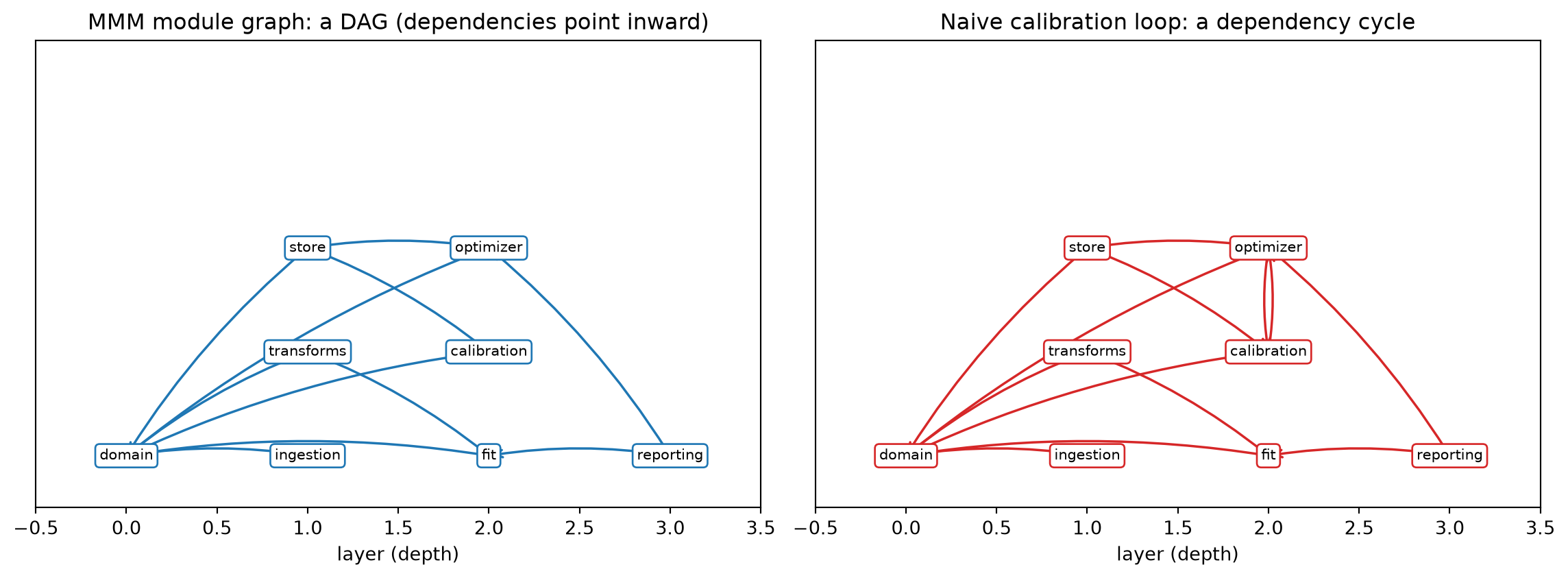
The single cell below builds the MMM module graph with nothing but the Python standard library and Matplotlib — no graph library — and runs the chapter’s three results. It computes each module’s instability and checks the Stable Dependencies Principle; it implements Kahn’s algorithm and confirms the build order; and it injects the naive calibration cycle, confirms the topological sort detects it, and confirms that routing through the store restores a DAG. The figure draws the dependency graph as an inward-pointing DAG alongside the version with the injected cycle.
from collections import dequeimport matplotlib.pyplot as plt# === 1. The MMM module dependency graph and instability metric (Rung 2 / WE1) ===# edge u -> v means "module u depends on module v"deps = {"domain": [],"ingestion": ["domain"],"transforms": ["domain"],"store": ["domain"],"fit": ["domain", "transforms"],"calibration": ["domain", "store"],"optimizer": ["domain", "store"],"reporting": ["fit", "optimizer"],}modules =list(deps)fan_out = {u: len(deps[u]) for u in modules}fan_in = {v: sum(v in deps[u] for u in modules) for v in modules}def instability(u): total = fan_in[u] + fan_out[u]return fan_out[u] / total if total else0.0I = {u: instability(u) for u in modules}print("1) Module instability (Stable Dependencies Principle)")print(f" {'module':12s} fan_in fan_out I")for u in modules:print(f" {u:12s}{fan_in[u]:6d}{fan_out[u]:7d}{I[u]:.2f}")assert I["domain"] ==0.0assert fan_in["domain"] ==max(fan_in.values())# Stable Dependencies Principle: every dependency points toward a no-less-stable moduleassertall(I[v] <= I[u] +1e-9for u in modules for v in deps[u])# === 2. Topological sort: Kahn's algorithm (Rung 3 / WE2) ===def kahn(graph): remaining = {u: len(graph[u]) for u in graph} # unmet dependencies dependents = {u: [] for u in graph}for u in graph:for v in graph[u]: dependents[v].append(u) ready = deque(u for u in graph if remaining[u] ==0) order = []while ready: x = ready.popleft() order.append(x)for w in dependents[x]: remaining[w] -=1if remaining[w] ==0: ready.append(w)return orderorder = kahn(deps)position = {u: i for i, u inenumerate(order)}print("\n2) Topological build order")print(" "+" -> ".join(order))assertlen(order) ==len(modules) # all placed => acyclicassertall(position[v] < position[u] for u in modules for v in deps[u]) # deps first# === 3. Cycle detection: break and fix the calibration loop (Rung 4 / WE3) ===bad = {u: list(vs) for u, vs in deps.items()}bad["optimizer"] = bad["optimizer"] + ["calibration"]bad["calibration"] = bad["calibration"] + ["optimizer"] # naive 2-cyclebad_order = kahn(bad)print("\n3) Calibration loop")print(f" naive optimizer<->calibration: {len(bad_order)} of {len(modules)} placed "f"-> cycle {'detected'iflen(bad_order) <len(modules) else'none'}")assertlen(bad_order) <len(modules)# Dependency Inversion: both depend on the stable store interface, not on each otherfixed = {u: list(vs) for u, vs in deps.items()} # already store-mediatedfixed_order = kahn(fixed)print(f" store-mediated (dependency inversion): {len(fixed_order)} of {len(modules)} placed -> DAG")assertlen(fixed_order) ==len(modules)# === Figure: the MMM dependency DAG vs the injected cycle (matplotlib only) ===layer = {"domain": 0, "ingestion": 1, "transforms": 1, "store": 1,"fit": 2, "calibration": 2, "optimizer": 2, "reporting": 3}within = {}pos = {}for u in modules: k = within.get(layer[u], 0); within[layer[u]] = k +1 pos[u] = (layer[u], k)def draw(ax, graph, title, color):for u in graph:for v in graph[u]: x0, y0 = pos[u]; x1, y1 = pos[v] ax.annotate("", xy=(x1, y1), xytext=(x0, y0), arrowprops=dict(arrowstyle="->", color=color, lw=1.3, connectionstyle="arc3,rad=0.08"))for u in modules: x, y = pos[u] ax.text(x, y, u, ha="center", va="center", fontsize=8, bbox=dict(boxstyle="round,pad=0.3", fc="white", ec=color)) ax.set_title(title); ax.set_xlabel("layer (depth)") ax.set_xlim(-0.5, 3.5); ax.set_ylim(-0.5, 4.0); ax.set_yticks([])fig, ax = plt.subplots(1, 2, figsize=(12, 4.5))draw(ax[0], deps, "MMM module graph: a DAG (dependencies point inward)", "tab:blue")draw(ax[1], bad, "Naive calibration loop: a dependency cycle", "tab:red")plt.tight_layout()plt.show()
1) Module instability (Stable Dependencies Principle)
   module       fan_in fan_out    I
   domain            6       0  0.00
   ingestion         0       1  1.00
   transforms        1       1  0.50
   store             2       1  0.33
   fit               1       2  0.67
   calibration       0       2  1.00
   optimizer         1       2  0.67
   reporting         0       2  1.00

2) Topological build order
   domain -> ingestion -> transforms -> store -> fit -> calibration -> optimizer -> reporting

3) Calibration loop
   naive optimizer<->calibration: 5 of 8 placed -> cycle detected
   store-mediated (dependency inversion): 8 of 8 placed -> DAG
The printed output confirms the chapter’s claims. The instability table reproduces WE1 exactly — domain at 0.00 with fan-in six, the leaves at 1.00 — and the Stable Dependencies check passes, every edge pointing toward stability. Kahn’s algorithm returns all eight modules in a valid build order, certifying the graph acyclic. Injecting the naive optimizer–calibration cycle drops the sort to five of eight modules, detecting the cycle, while the store-mediated version sorts all eight — Dependency Inversion turning the runtime loop into an acyclic dependency graph. The figure shows the inward-pointing DAG beside the version whose two red back-edges close the cycle.
24.5 Exercises
24.5.1 C – Conceptual / Reading Comprehension
C1. Explain why an acyclic dependency graph permits a system to be built and unit-tested one module at a time, while a cycle does not. What, concretely, goes wrong when you try to build or test a module that lies on a dependency cycle?
C2. The Stable Dependencies Principle says dependencies should point toward more stable (lower-instability) modules. Explain the asymmetry of risk that motivates it: what happens when a volatile module depends on a stable one, versus when a stable module depends on a volatile one?
C3. The calibration–optimization loop is, in one sense, a cycle and, in another, not. Name the sense in which it cycles and the sense in which it does not, and explain how the prior-store interface lets both be true at once.
24.5.2 B – By Hand
B1. A system has modules with dependencies a→b, a→c, b→d, c→d, d depends on nothing. Compute fan-in, fan-out, and the instability I of each module, and identify the most and least stable.
B2. Produce a topological (build) order for the graph of B1 by hand, naming the rule you use at each step.
B3. Suppose an edge d→a is added to the B1 graph. Show that no topological order exists by attempting Kahn’s algorithm and identifying the modules that can never be placed.
24.5.3 P – Prove It
P1. Prove that a finite directed graph admits a topological order if and only if it is acyclic. Give both directions; for the “acyclic implies an order exists” direction, give the constructive argument (Kahn’s algorithm) and justify why a vertex of out-degree zero must exist at each step.
P2. Two modules A and B depend on each other (A \to B and B \to A), forming a 2-cycle. Prove that introducing a single new module C with A \to C and B \to C, and removing the two original edges, yields an acyclic graph. (Dependency Inversion.)
24.5.4 A – Applied / Code
A1. Write a function that, given any dependency dictionary, returns a topological order if one exists or otherwise reports the set of modules involved in (or downstream of) a cycle. Run it on the MMM graph with and without the optimizer–calibration loop edges.
A2. Write a function that computes each module’s instability and returns every dependency edge u → v that violates the Stable Dependencies Principle (those with I(v) > I(u)). Confirm the MMM graph has none, then add a violating edge and confirm it is flagged.
24.6 Summary
This chapter architected the MMM system as a directed graph of modules and dependencies, and reduced “good architecture” to a single structural property with a single theorem behind it. Coupling and cohesion are made countable through fan-in and fan-out; Martin’s instability metric turns those counts into a measure of how safely each module can change, and the Stable Dependencies Principle says dependencies must point toward the stable core. The keystone is that the dependency graph admits a build-and-test order exactly when it is acyclic — so acyclicity is precisely the condition for building, testing, and replacing components independently. The apparent cycle of the Part VI calibration–optimization loop dissolves under the Dependency Rule: a runtime data cycle need not be a source-code dependency cycle, because routing both the optimizer and calibration through the stable prior-store interface keeps the module graph acyclic. The resulting inward-pointing layered architecture is what makes the system maintainable, and it sets up the prior store as a built data product (Chapter 25) and the testing it enables (Chapter 26).
Key concepts.
Information hiding. A module exposes an interface and conceals its implementation, so consumers depend on what it does, not how — letting the implementation change locally.
Coupling and cohesion. Cohesion (relatedness within a module) should be high and coupling (dependence between modules) low; fan-in and fan-out make coupling countable.
Instability and the Stable Dependencies Principle.I = \text{fan-out}/(\text{fan-in} + \text{fan-out}) measures exposure to change; dependencies should point toward lower-instability modules, confining volatility to the periphery.
Acyclicity is buildability. A dependency graph can be built and tested one module at a time exactly when it is acyclic; a cycle entangles its modules so none can be isolated.
The Dependency Rule. A runtime data cycle is not a source-code dependency cycle; routing interaction through a stable interface (Dependency Inversion) keeps the module graph acyclic regardless of data flow.