Motivation
Chapter 16 closed a loop: given the data-generating process from Chapter 15 and a Bayesian inference engine assembled from Chapters 5, 9, and 11, it recovered the adstock decay, saturation curve, and channel coefficients that produced a synthetic sales series. The model that made that recovery possible assumed constant coefficients — the effectiveness of each channel, \beta_i, was treated as a fixed number to be learned from the full time series at once. That assumption is a defensible starting point, but it is a falsifiable null, not a law of marketing. Media efficiency decays as audiences habituate to a creative. Targeting algorithms shift reach pools as platform inventory fluctuates. Brand equity builds and erodes on timescales of months. A channel that drove strong returns in the first two quarters of a campaign may be near saturation by the fourth. A constant \beta_i averages over this drift; it cannot distinguish a channel that was equally effective across all periods from one that was effective early and exhausted later. The practical cost is real: a model that pools effectiveness across time misprices the present, misattributes the recent, and gives budget recommendations anchored to an average that may describe no actual period in the data.
The dynamic linear model (DLM) relaxes the constant-coefficient assumption while preserving tractable inference. The key move is to treat the coefficient vector as a latent state that evolves through time — \theta_t rather than \theta — and to model two layers simultaneously: a state equation that describes how the coefficient vector drifts from one period to the next, and an observation equation that links the current state to the observed sales through the familiar structural equation. In matrix form,
\begin{aligned}
\theta_t &= G_t\, \theta_{t-1} + w_t, \qquad w_t \sim \mathcal{N}(0,\, W_t), \\
y_t &= F_t^\top \theta_t + v_t, \qquad v_t \sim \mathcal{N}(0,\, V_t),
\end{aligned}
where F_t is the vector of regressors at time t (adstocked spend, baseline components), G_t is the evolution matrix (often the identity for a local-level random walk), and W_t, V_t are the state and observation noise covariances. The coefficients are never observed directly; they are inferred from the noisy sales signal y_t. When G_t = I and the variances are small, the states move slowly and the model behaves like its constant-coefficient cousin; as W_t grows, the model allows faster drift and the effective information per period shrinks. The DLM encodes the modeler’s prior belief about how quickly channel effectiveness changes, and the data update that belief period by period.
This is the time-series payoff that Chapter 7 pointed toward but could not yet deliver. That chapter showed that AR(1) dynamics and adstock carryover are both first-order recursions — linear maps applied one step at a time to a scalar state. State-space models generalize that structure to the regression coefficients themselves: the coefficient vector at time t is a linear function of its value at time t-1, perturbed by Gaussian noise, exactly as the adstock recursion a_t = \lambda\, a_{t-1} + x_t carries media exposure forward. The DLM’s state equation \theta_t = G_t\,\theta_{t-1} + w_t applies the same logic to the full parameter vector. The two ideas — carry-forward of media exposure and carry-forward of marketing effectiveness — are now expressed in the same mathematical language, and the distinction between them is a matter of what enters the state rather than how the state evolves.
The chapter’s internal structure repeats the book’s earlier frequentist-to-Bayesian arc. Chapters 4 and 5 introduced linear regression first as an ordinary-least-squares problem and then as a Bayesian conditioning problem, showing that the two formulations coincide under Gaussian noise. This chapter runs the same arc at the time-series level. The classical Kalman filter derives the minimum-variance linear estimator of the latent state at each period by recursively applying Gaussian conditioning (Chapters 3 and 5) — no sampling, no approximation, just the analytic consequence of multiplying Gaussians. The Bayesian DLM then places prior distributions on the variance parameters and recovers the full posterior by appending a backward smoothing pass — the forward-filtering backward-sampling (FFBS) algorithm of West and Harrison (1997) — that draws joint samples from the state sequence. With variances fixed and known, the Kalman recursions are the exact posterior: conjugacy closes completely. Make the variances unknown and the conjugacy breaks; the marginal posterior over the variance parameters has no closed form, and you are back to Gibbs sampling (Chapters 6 and 9), alternating between a closed-form state draw from the Kalman smoother and an MCMC draw over the variances. The DLM is the book’s cleanest illustration of where conjugacy ends and sampling must begin.
The machinery developed here reaches forward into the book’s final arc. Chapter 20’s causal counterfactuals — estimating what sales would have been absent a spend change — rest on the Kalman filter’s ability to project latent states forward under an alternative scenario; the DLM provides the model that makes those projections probabilistically calibrated. Chapter 22’s prior store extracts the posterior distributions over channel effectiveness from a fitted DLM and recycles them as informative priors in future campaigns, closing the loop between inference and planning. The advanced production reframing of the DLM for time-varying coefficient MMM deployment is flagged at the chapter’s close as an optional endpoint for readers who want to carry these ideas directly into practice.
Theory & Proofs
The theory develops in two rungs. Rung 1 motivates the generalization: the constant-coefficient model of Chapter 16 is a falsifiable null, and promoting the fixed coefficient vector to a time-indexed latent state is the precise way to relax it. Rung 2 formalizes that commitment as the state-space pair, names every component, and exhibits the two anchor DLMs the chapter uses throughout.
Rung 1 — Static to dynamic
Chapter 16 demonstrated that Bayesian inference can recover the adstock decay, saturation curve, and channel coefficients from a well-designed campaign. It did so by treating every channel coefficient \beta_i as a fixed scalar, constant across the entire observation window. That assumption is not merely a convenience; it is a falsifiable empirical claim. A channel that drove 2\times ROI in January is assumed to drive 2\times ROI in December, after a full year of audience exposure, creative repetition, and inventory pressure. The claim can be wrong — and in practice, it often is. Media efficiency decays as audiences habituate to a creative (wear-out). Targeting algorithms shift reach pools as platform inventory fluctuates. Brand equity builds and erodes on timescales that cut across campaign periods. When true channel effectiveness drifts, a constant-\beta model pools across the drift and estimates an average that may describe no actual period in the data: recent periods look underfit, early periods look overfit, and budget recommendations are anchored to a number the business has already departed from.
This chapter relaxes the constant-\beta assumption one layer deeper than Chapter 7’s AR(1) extension. Chapter 7 relaxed the assumption that residuals are i.i.d. — it allowed the unexplained variation in sales to carry its own temporal structure — while regression coefficients remained fixed. This chapter relaxes the assumption that regression coefficients themselves are fixed. The modeling commitment is precise: promote the fixed coefficient vector \theta to a time-indexed latent state \theta_t. Each period, \theta_t takes a value that may differ from its predecessor; the observed sales y_t is a noisy measurement of the structural equation evaluated at that period’s state. Because \theta_t is never observed directly, the model must simultaneously infer how it evolves and what value it must have taken to be consistent with the observed y_t. That dual inference — tracking a hidden state while explaining a noisy measurement — is the state-space problem.
Rung 2 — The state-space form
The DLM encodes the Rung 1 commitment in two equations. Let y_t \in \mathbb{R} denote observed sales at period t, \theta_t \in \mathbb{R}^p the latent state, F_t \in \mathbb{R}^p the observation vector, and G_t \in \mathbb{R}^{p \times p} the evolution matrix. The model is
\begin{aligned}
y_t &= F_t^\top \theta_t + v_t, \qquad v_t \sim \mathcal{N}(0,\, V_t), \\
\theta_t &= G_t \theta_{t-1} + w_t, \qquad w_t \sim \mathcal{N}(0,\, W_t),
\end{aligned}
with the two noise sequences independent of each other and across time. The components have precise roles.
- \theta_t: the latent state — the time-varying coefficient vector (channel effectiveness, baseline level, trend) that summarizes the system’s condition at period t.
- F_t: the observation (design) vector — the regressors at time t, including adstocked channel spend and any baseline components; observed and controlled by the analyst.
- G_t: the evolution (state-transition) matrix — it propagates \theta_{t-1} forward one period, encoding the assumed dynamic structure of the coefficient process.
- V_t: the observation-noise variance — the variance of the deviation between the structural mean F_t^\top \theta_t and the realized sales y_t.
- W_t: the state-evolution (drift) covariance — the variance of the perturbation that moves the coefficient vector from one period to the next; its magnitude sets how fast the model allows coefficients to change.
Anchor model 1 — Local level. Set F = G = 1 (scalar model, p = 1). The pair reduces to
\begin{aligned}
y_t &= \theta_t + v_t, \\
\theta_t &= \theta_{t-1} + w_t,
\end{aligned}
a random walk observed in noise. This is the simplest DLM: no regressors, one evolving level. It is the lens through which the chapter derives the steady-state Kalman gain, because the single ratio W/V completely determines how fast the filter adapts — making the effect of state drift versus observation noise visible in isolation before any regression structure is added.
Anchor model 2 — Regression DLM. Set F_t = x_t (the adstocked spend of one channel at period t) and G = I. The state equation reduces to \beta_t = \beta_{t-1} + w_t — a random walk on the channel coefficient — and the observation equation becomes
y_t = x_t \beta_t + v_t.
This is the time-varying-coefficient MMM the chapter fits. The coefficient \beta_t absorbs everything the constant-\beta model averaged over: wear-out, audience shift, and efficiency recovery after a creative rotation. Dividing the recovered \beta_t by the channel’s cost-per-unit gives a time-varying cost-per-revenue that the planner can track and respond to within the campaign window. Multiple channels extend the model by stacking adstocked spend into the vector F_t = x_t and coefficients into \theta_t, with G = I_p keeping each channel’s random walk independent.
The ratio W/V — state drift relative to observation noise — governs how quickly the model allows coefficients to move: a large ratio permits fast adaptation at the cost of noisier period-by-period estimates; a small ratio anchors the model close to a constant-\beta solution, and setting it is the practitioner’s primary tuning decision.
Rung 3 — The Kalman filter
The state-space form of Rung 2 defines the model but does not yet provide inference. Given observations y_1, y_2, \ldots, y_T and known noise covariances V_t and W_t, the goal is to recover the filtering distribution p(\theta_t \mid y_{1:t}) — the posterior over the latent state at period t, conditioned on all data through that period. The Kalman filter accomplishes this by a two-step forward recursion that converts the posterior at period t-1 into the posterior at period t.
Predict step. Start from the filtered posterior at the previous period, \theta_{t-1} \mid y_{1:t-1} \sim \mathcal{N}(m_{t-1}, C_{t-1}). Push the state through the evolution equation \theta_t = G_t \theta_{t-1} + w_t. Because this is an affine transformation of a Gaussian with independent Gaussian noise w_t \sim \mathcal{N}(0, W_t) added, the one-step-ahead prior over \theta_t given y_{1:t-1} is Gaussian with
a_t = G_t m_{t-1}, \qquad R_t = G_t C_{t-1} G_t^\top + W_t.
Update step. When y_t arrives, condition on it. The observation equation y_t = F_t^\top \theta_t + v_t is affine in \theta_t with independent Gaussian noise, so the pair (\theta_t, y_t) is jointly Gaussian given y_{1:t-1}. Applying the conditional-Gaussian formula (Chapters 3 and 5) yields the filtered posterior \theta_t \mid y_{1:t} \sim \mathcal{N}(m_t, C_t), where
m_t = a_t + A_t (y_t - f_t), \qquad C_t = R_t - A_t Q_t A_t^\top, \qquad A_t = R_t F_t Q_t^{-1},
f_t = F_t^\top a_t is the one-step-ahead forecast mean, Q_t = F_t^\top R_t F_t + V_t is the forecast variance, and the Kalman gain A_t weights the innovation y_t - f_t by the relative informativeness of the observation. With known (V_t, W_t), these two steps together return the exact Gaussian filtering posterior p(\theta_t \mid y_{1:t}) at every period in closed form — no sampling, no approximation. Proof P1 formalizes this claim.
Proof P1 — Kalman filter as exact Gaussian conditioning (keystone)
Proposition P1. For the DLM with known V_t, W_t, if \theta_{t-1} \mid y_{1:t-1} \sim \mathcal{N}(m_{t-1}, C_{t-1}) then \theta_t \mid y_{1:t} \sim \mathcal{N}(m_t, C_t) with the recursions below; hence the filtering distribution is Gaussian at every t.
Proof. By induction on t.
Inductive hypothesis. \theta_{t-1} \mid y_{1:t-1} \sim \mathcal{N}(m_{t-1}, C_{t-1}).
Predict. The evolution equation \theta_t = G_t \theta_{t-1} + w_t is an affine-Gaussian map: G_t applied to a Gaussian random vector with independent Gaussian noise w_t \sim \mathcal{N}(0, W_t) added. By the standard affine-transformation and addition rules for Gaussians, the one-step-ahead prior is
\theta_t \mid y_{1:t-1} \sim \mathcal{N}(a_t,\, R_t), \qquad a_t = G_t m_{t-1}, \quad R_t = G_t C_{t-1} G_t^\top + W_t.
Joint of state and next observation. Since y_t = F_t^\top \theta_t + v_t is affine-Gaussian in \theta_t and v_t \sim \mathcal{N}(0, V_t) is independent of \theta_t \mid y_{1:t-1}, the pair (\theta_t, y_t) given y_{1:t-1} is jointly Gaussian. Compute each block of the joint covariance:
\begin{aligned}
\mathbb{E}[y_t \mid y_{1:t-1}] &= F_t^\top a_t \;\equiv\; f_t, \\
\mathrm{Var}(y_t \mid y_{1:t-1}) &= F_t^\top R_t F_t + V_t \;\equiv\; Q_t, \\
\mathrm{Cov}(\theta_t, y_t \mid y_{1:t-1}) &= \mathrm{Cov}(\theta_t,\, F_t^\top \theta_t + v_t \mid y_{1:t-1}) = R_t F_t,
\end{aligned}
where the last line uses independence of v_t from \theta_t and \mathrm{Cov}(\theta_t, F_t^\top \theta_t \mid y_{1:t-1}) = \mathbb{E}[(\theta_t - a_t)(\theta_t - a_t)^\top \mid y_{1:t-1}]\, F_t = R_t F_t. Assembling the blocks:
\begin{bmatrix} \theta_t \\ y_t \end{bmatrix} \Bigm| y_{1:t-1} \sim \mathcal{N}\!\left( \begin{bmatrix} a_t \\ f_t \end{bmatrix},\ \begin{bmatrix} R_t & R_t F_t \\ F_t^\top R_t & Q_t \end{bmatrix} \right).
Update by Gaussian conditioning. Apply the conditional-Gaussian formula (Chapters 3 and 5): for a joint Gaussian with blocks \Sigma_{uu}, \Sigma_{uz}, \Sigma_{zz}, the conditional distribution of u given z has mean \mu_u + \Sigma_{uz} \Sigma_{zz}^{-1}(z - \mu_z) and covariance \Sigma_{uu} - \Sigma_{uz} \Sigma_{zz}^{-1} \Sigma_{zu}. Identifying u = \theta_t, z = y_t, \Sigma_{uz} = R_t F_t, \Sigma_{zz} = Q_t:
m_t = a_t + A_t (y_t - f_t), \qquad C_t = R_t - A_t Q_t A_t^\top, \qquad A_t = R_t F_t Q_t^{-1}.
The Kalman gain A_t weights the innovation y_t - f_t by the relative informativeness of the observation. This shows \theta_t \mid y_{1:t} \sim \mathcal{N}(m_t, C_t), closing the induction. \blacksquare
With (V_t, W_t) known these are exact closed-form updates — conjugacy doing all the work, no sampling — the point Proof P3 will revisit.
Rung 4 — The RTS smoother
The Kalman filter produces, at each period t, the filtering distribution \mathcal{N}(m_t, C_t) — the posterior over \theta_t conditioned on observations up through that period, y_{1:t}. It does so by a strictly forward pass: at time t the filter has not yet seen y_{t+1}, \ldots, y_T. The Rauch–Tung–Striebel (RTS) smoother revisits each state after the forward pass is complete, conditioning on the full data set y_{1:T} to produce the smoothing distribution p(\theta_t \mid y_{1:T}) = \mathcal{N}(m_t^s, C_t^s).
Because future observations are informative about the current state through the chain of evolution equations, incorporating them always tightens the posterior: C_t^s \preceq C_t (positive semi-definite ordering) at every t. The smoother cannot be worse than the filter, and it is strictly better for any interior time point where at least one future observation has been withheld by the filter.
The RTS backward recursion is initialized at the final filtered distribution, m_T^s = m_T and C_T^s = C_T, and then runs backward from t = T-1 to t = 0. For the random-walk evolution G = I:
B_t = C_t R_{t+1}^{-1}, \qquad m_t^s = m_t + B_t\,(m_{t+1}^s - a_{t+1}), \qquad C_t^s = C_t + B_t\,(C_{t+1}^s - R_{t+1})\,B_t^\top.
Here B_t is the smoother gain — the fraction of the one-step-ahead uncertainty R_{t+1} that the filtered uncertainty C_t can explain. The correction m_{t+1}^s - a_{t+1} is the difference between the smoothed mean one step ahead and the Kalman one-step-ahead forecast; it propagates information from the future back into the current state. The term C_{t+1}^s - R_{t+1} is non-positive definite (the smoothed variance is no larger than the predicted variance), so the correction to C_t^s is non-positive, confirming that smoothing cannot inflate uncertainty. The full derivation of the backward recursion — showing it arises from exactly the same conditional-Gaussian formula used in Proof P1, applied to the joint of \theta_t and \theta_{t+1} given y_{1:t} — is left as a P-tier exercise.
Rung 5 — Bayesian DLM and FFBS
The Kalman filter and RTS smoother of Rungs 3 and 4 treat the noise variances V_t and W_t as known. In practice they must be estimated, and the fully Bayesian treatment places prior distributions on (\theta_0, V, W) — the initial state, the observation noise variance, and the state-drift covariance — and targets the joint posterior over both the state sequence and the variance parameters:
p(\theta_{0:T}, V, W \mid y_{1:T}).
This joint posterior has no closed form. The Markov structure of the state sequence — the fact that \theta_t depends on the past only through \theta_{t-1}, and on future data only through \theta_{t+1} — suggests a Gibbs sampler (Ch. 6, Ch. 9) that alternates between two conditionally conjugate blocks:
- Draw the full state path given the variances. With V and W fixed, the state sequence \theta_{0:T} is a Gaussian hidden Markov model, and its joint posterior is the output of forward-filtering backward-sampling (FFBS).
- Draw the variances given the full state path. With \theta_{0:T} fixed, the observation residuals y_t - F_t^\top \theta_t and the evolution increments \theta_t - G_t \theta_{t-1} are observed, and conjugate inverse-gamma priors on V and W yield closed-form inverse-gamma updates.
FFBS is “the Kalman filter you already know, run forward, then sampled backward.” It proceeds in two passes.
Forward pass. Run the Kalman filter from t = 1 to t = T, storing all intermediate quantities: the one-step-ahead means and covariances (a_t, R_t) and the filtered means and covariances (m_t, C_t). The forward pass is identical to Rung 3; no additional computation is required.
Backward sampling pass. Draw \theta_T \sim \mathcal{N}(m_T, C_T), the final filtered posterior. Then, for t = T-1, T-2, \ldots, 0, draw each state from its backward conditional distribution
\theta_t \mid \theta_{t+1}, y_{1:t} \sim \mathcal{N}\!\left(m_t + B_t(\theta_{t+1} - a_{t+1}),\; C_t - B_t R_{t+1} B_t^\top\right),
where B_t = C_t G_{t+1}^\top R_{t+1}^{-1}, using the stored filter quantities. Because each draw conditions on the already-sampled \theta_{t+1}, the path is generated in reverse and each draw is a single sample from a Gaussian — O(p^3) per step for the Cholesky of the p \times p conditional covariance. The full state path \theta_{0:T} is an exact sample from the joint smoothing posterior; Proof P2 establishes why.
Inside the Gibbs loop, FFBS and the conjugate variance updates alternate. Each full cycle produces one draw from the joint posterior p(\theta_{0:T}, V, W \mid y_{1:T}), and the Gibbs convergence guarantees of Ch. 9 apply.
Proof P2 — FFBS correctness
Proposition P2. FFBS draws an exact sample from the joint smoothing posterior p(\theta_{0:T} \mid y_{1:T}).
Proof.
Factorization via the Markov property. The state sequence \theta_{0:T} satisfies the Markov property: \theta_t depends on the past only through \theta_{t-1}, and on the observations only through the observations available at time t and the future states. Precisely, given \theta_{t+1}, the state \theta_t is conditionally independent of the future data y_{t+1:T}, because those observations influence \theta_t only through the chain \theta_t \to \theta_{t+1} \to \cdots, which is blocked by conditioning on \theta_{t+1}. Applying this to the joint smoothing posterior by the chain rule of probability:
p(\theta_{0:T} \mid y_{1:T}) = p(\theta_T \mid y_{1:T}) \prod_{t=0}^{T-1} p(\theta_t \mid \theta_{t+1},\, y_{1:t}).
Each factor is Gaussian. The terminal factor p(\theta_T \mid y_{1:T}) = \mathcal{N}(m_T, C_T) is the final filtered posterior, produced by the Kalman forward pass (Proof P1). Each backward factor p(\theta_t \mid \theta_{t+1}, y_{1:t}) is a Gaussian conditioning problem: starting from the filtered distribution \theta_t \mid y_{1:t} \sim \mathcal{N}(m_t, C_t) and the evolution link \theta_{t+1} = G_{t+1} \theta_t + w_{t+1}, the pair (\theta_t, \theta_{t+1}) given y_{1:t} is jointly Gaussian with
\begin{aligned}
\mathbb{E}[\theta_{t+1} \mid y_{1:t}] &= G_{t+1} m_t = a_{t+1}, \\
\mathrm{Var}(\theta_{t+1} \mid y_{1:t}) &= G_{t+1} C_t G_{t+1}^\top + W_{t+1} = R_{t+1}, \\
\mathrm{Cov}(\theta_t, \theta_{t+1} \mid y_{1:t}) &= C_t G_{t+1}^\top.
\end{aligned}
Applying the conditional-Gaussian formula (Chapters 3 and 5) — the same formula used in Proof P1 — gives
\theta_t \mid \theta_{t+1}, y_{1:t} \sim \mathcal{N}\!\left(m_t + B_t(\theta_{t+1} - a_{t+1}),\; C_t - B_t R_{t+1} B_t^\top\right), \quad B_t = C_t G_{t+1}^\top R_{t+1}^{-1}.
Conclusion. The joint smoothing posterior factors into a product of Gaussians, each computable from the stored Kalman filter quantities. Drawing \theta_T \sim \mathcal{N}(m_T, C_T) and then each \theta_t backward from its Gaussian conditional, using the already-drawn \theta_{t+1}, samples exactly from the factored joint, which equals p(\theta_{0:T} \mid y_{1:T}). \blacksquare
Rung 6 — The conjugacy-vs-MCMC boundary
Proofs P1 and P2 together establish the DLM’s central lesson. With variances V and W fixed and known, the Kalman recursions are the exact posterior: no sampling, no approximation, just closed-form Gaussian conditioning carried forward one step at a time. Conjugacy does all the work because the model is a product of Gaussians linked by affine maps, and the space of Gaussian distributions is closed under those operations. Making the variances unknown breaks the closure: placing prior distributions on V and W couples the state sequence and the variance parameters in a way that leaves the joint posterior with no closed form. Closed-form inference is no longer possible; MCMC is required. This is the book’s sharpest illustration of where conjugacy ends and sampling must begin — sharper than the logistic regression of Ch. 5 or the hierarchical variance of Ch. 6, because here the boundary is explicit: it is the line between known and unknown (V, W).
Proof P3 — Known variances ⇒ closed form; unknown ⇒ MCMC
Proposition P3. With the DLM of Rung 2: (i) if V and W are known, the filtered posteriors and the marginal likelihood p(y_{1:T}) are available in closed form; (ii) if V and W are unknown with prior distributions assigned, the joint posterior p(\theta_{0:T}, V, W \mid y_{1:T}) has no closed form, and a Gibbs sampler restores tractability.
Proof.
Part 1 — Known (V, W). By Proof P1, \theta_t \mid y_{1:t} \sim \mathcal{N}(m_t, C_t) at every t, with recursions that are finite compositions of affine-Gaussian operations on a starting Gaussian — exact and closed-form. The marginal likelihood p(y_{1:T}) factors through the one-step-ahead predictive distributions via the prediction-error (innovations) decomposition:
p(y_{1:T}) = \prod_{t=1}^{T} p(y_t \mid y_{1:t-1}) = \prod_{t=1}^{T} \mathcal{N}(y_t;\, f_t,\, Q_t),
since each y_t \mid y_{1:t-1} is the Gaussian forecast produced by the filter with mean f_t = F_t^\top a_t and variance Q_t = F_t^\top R_t F_t + V. The product of Gaussian densities evaluated at the observed data is a closed-form function of (V, W) — it can be maximized directly (classical maximum-likelihood estimation of the variance parameters, no sampling required).
Part 2 — Unknown (V, W). Place prior distributions on (V, W) — for concreteness, conjugate inverse-gamma priors. The joint posterior is
p(\theta_{0:T}, V, W \mid y_{1:T}) \;\propto\; p(V)\,p(W)\,p(\theta_0)\prod_{t=1}^{T} p(y_t \mid \theta_t, V)\,p(\theta_t \mid \theta_{t-1}, W).
The quantities R_t and Q_t that enter the filtering recursions (Proof P1) depend on W and V respectively. Marginalizing over \theta_{0:T} to obtain p(V, W \mid y_{1:T}) requires integrating out a product of T Gaussian terms whose covariance matrices are nonlinear functions of (V, W); this integral has no closed form. Conjugacy is broken.
A Gibbs sampler (Ch. 6, Ch. 9) restores tractability by separating the state and variance blocks:
- Draw \theta_{0:T} \mid V, W, y_{1:T}: with (V, W) fixed, this is exactly Proof P2 — FFBS produces an exact sample from the joint smoothing posterior p(\theta_{0:T} \mid V, W, y_{1:T}), a product of Gaussians.
- Draw V \mid \theta_{0:T}, y_{1:T}: with \theta_{0:T} fixed, the observation residuals e_t = y_t - F_t^\top \theta_t are observed. Under an inverse-gamma prior V \sim \operatorname{Inv-Gamma}(a_V, b_V), the sufficient statistic is the sum of squared residuals \sum_t e_t^2, and the posterior is V \mid \theta_{0:T}, y \sim \operatorname{Inv-Gamma}\!\left(a_V + T/2,\; b_V + \tfrac{1}{2}\sum_{t=1}^{T} e_t^2\right) — closed-form.
- Draw W \mid \theta_{0:T}, y_{1:T}: with \theta_{0:T} fixed, the state increments \delta_t = \theta_t - G_t \theta_{t-1} are observed. Under an inverse-Wishart (or inverse-gamma if W is scalar) prior, the sufficient statistic is \sum_t \delta_t \delta_t^\top, and the posterior is conjugate and closed-form.
Each full Gibbs cycle yields an exact draw from the respective conditional. The Gibbs convergence guarantees of Ch. 9 apply, and the resulting chain targets p(\theta_{0:T}, V, W \mid y_{1:T}). This is exactly where conjugacy ends and MCMC begins. \blacksquare
Rung 7 — Bayesian time-varying coefficients
Advanced / Extensions (skippable). The core chapter ends here. This section sketches a production reframing of time-varying coefficients; it is not required for anything that follows. The full mechanics are deferred to the appendix.
The DLM’s random-walk state equation evolves one coefficient per period, producing a trajectory \theta_{0:T} with as many free vectors as there are time steps. A production reframing due to Ng et al. (2021) — Bayesian time-varying coefficients (BTVC) — replaces this per-step state with J \ll T latent knots, assembled into a coefficient trajectory via a kernel smoother: \beta = Kb, where K is a fixed T \times J smoothing matrix and b \in \mathbb{R}^J is the vector of knot values. The parameter count decouples from the series length: doubling T does not double the model’s free parameters, it only changes which portion of the trajectory each observation informs. A folded-normal two-layer hierarchy enforces non-negativity and shrinkage of the channel coefficients, replacing the DLM’s unconstrained Gaussian state with a prior structure that is anchored at zero from below.
The trade is direct: BTVC gives up the DLM’s exact Kalman recursions in exchange for scalability and built-in positivity constraints. The FFBS sampler of Proof P2 is replaced by stochastic variational inference — a fast, optimization-based approximation to the posterior that scales to long series and many channels without the O(T) Markov-chain burn-in of MCMC. The approximation introduces a gap between the true posterior and the variational family, a cost the DLM does not pay; the DLM’s exact recursions are not approximate in this sense. Which trade is worth making depends on the modeling context: BTVC is the natural endpoint when positivity and computational scale are the binding constraints, and the DLM is the natural choice when exact posterior propagation matters. The full mechanics of the knot parameterization, the folded-normal hierarchy, and the variational objective are developed in the appendix.
Worked Examples
Three worked examples carry the chapter’s main results into arithmetic — one tracing the Kalman recursion to its steady-state fixed point and identifying the golden ratio, one demonstrating the filter–smoother gap on a drifting coefficient, and one placing the two inference regimes of Proof P3 side by side on the same series.
WE1 — Local-level steady-state Kalman gain (the golden ratio)
Setup.
Local-level model: F = G = 1, V = W = 1. Start from m_0 = 0, C_0 = 0 — a completely uninformative initial condition.
One predict–update cycle.
Predict:
a_1 = G\,m_0 = 0, \qquad R_1 = G\,C_0\,G^\top + W = 0 + 1 = 1.
Forecast:
f_1 = F^\top a_1 = 0, \qquad Q_1 = F^\top R_1 F + V = 1 + 1 = 2.
Kalman gain and updated variance:
A_1 = R_1\,F\,Q_1^{-1} = \frac{1}{2}, \qquad C_1 = R_1 - A_1\,Q_1\,A_1^\top = 1 - \frac{1}{2}\cdot 2\cdot\frac{1}{2} = \frac{1}{2}.
The first observation halves the prior variance. Continuing: R_2 = C_1 + W = 1.5, Q_2 = R_2 + V = 2.5, A_2 = 0.6, C_2 = 1.5 - (0.6)(2.5)(0.6) = 0.6. The sequence C_t is decreasing and bounded below; it converges to a fixed point.
The variance recursion and its fixed point.
The filtered variance satisfies C_{t+1} = (C_t + W) - (C_t + W)^2/(C_t + W + V). Substituting R = C + W for the one-step-ahead variance, at the fixed point C^* = R^* - W the recursion gives
R^* - W = R^* - \frac{(R^*)^2}{R^* + V} \qquad \Longrightarrow \qquad W(R^* + V) = (R^*)^2.
With W = V = 1:
(R^*)^2 - R^* - 1 = 0,
whose positive root is
R^* = \frac{1 + \sqrt{5}}{2} = \varphi \approx 1.618,
the golden ratio. The steady-state Kalman gain follows immediately:
K^\star = \frac{R^*}{R^* + V} = \frac{\varphi}{\varphi + 1} = \frac{\sqrt{5} - 1}{2} \approx 0.6180.
Interpretation.
The steady-state filter is an exponentially-weighted moving average with smoothing constant K^\star \approx 0.618: each new observation gets weight 0.618 and the running estimate gets weight 0.382. The golden-ratio appearance is not a coincidence — it is the exact consequence of setting W = V, which forces the characteristic equation R^2 - R - 1 = 0 that defines \varphi. As W/V increases (state drifts faster relative to observation noise), K^\star \to 1 and the filter discards its history entirely; as W/V \to 0 (nearly static level), K^\star \to 0 and the estimate barely moves. The ratio W/V is the single free parameter controlling adaptation speed in the local-level model, and the steady-state gain is its closed-form summary.
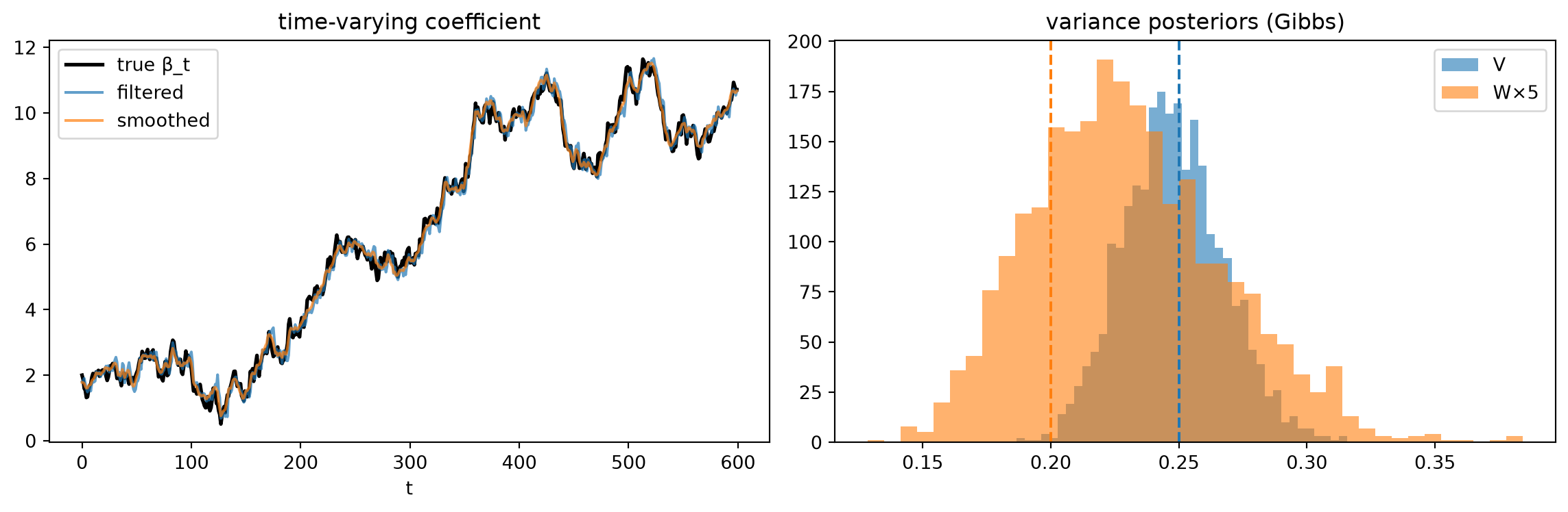
WE2 — Regression DLM: recovering a drifting coefficient
Setup.
Single channel with a time-varying coefficient \beta_t following a random walk: \beta_t = \beta_{t-1} + w_t with state variance W = 0.04. The observation equation is y_t = x_t \beta_t + v_t with observation variance V = 0.25, over T = 600 weeks.
Kalman filter: tracking forward.
Running the Kalman filter forward from a diffuse prior produces, at each t, the filtering distribution \beta_t \mid y_{1:t} \sim \mathcal{N}(m_t, C_t). The filter has access only to data through the current period — it cannot look ahead. Against the true \beta_t trajectory used to generate the series, the filter achieves RMSE \approx 0.27.
RTS smoother: conditioning on the full series.
Running the RTS backward recursion from t = T down to t = 1 — each step incorporating the information in all future observations through the smoother gain B_t = C_t R_{t+1}^{-1} — produces the smoothing distributions \beta_t \mid y_{1:T} \sim \mathcal{N}(m_t^s, C_t^s). Because the smoother has access to the whole series, C_t^s \le C_t at every interior period: the backward pass can only tighten, never widen, posterior uncertainty. The smoother achieves RMSE \approx 0.20, a roughly 25% improvement over the filter.
| Kalman filter |
\approx 0.27 |
| RTS smoother |
\approx 0.20 |
What \beta_t represents.
The recovered \beta_t is the channel’s time-varying marginal revenue per unit of adstocked spend — its effectiveness curve over the campaign. A constant-\beta model averages over this trajectory and reports a single number that may describe no actual period; the DLM surfaces the full curve. The smoother’s estimate, tighter than the filter’s, is the right summary quantity for retrospective attribution over a completed campaign; the filter’s estimate, available period by period as data arrive, is the right quantity for real-time budget pacing.
WE3 — The same model, two inference regimes
Setup.
Same series as WE2: T = 600, V = 0.25, W = 0.04.
Regime 1 — Known (V, W): closed-form marginal likelihood.
With V and W known, Proof P3 Part 1 supplies the exact marginal likelihood via the prediction-error decomposition:
\log p(y_{1:T}) = \sum_{t=1}^{T} \log \mathcal{N}(y_t;\, f_t,\, Q_t).
Each term is a Gaussian log-density evaluated at the observed y_t, with one-step-ahead mean f_t = x_t a_t and variance Q_t = x_t^2 R_t + V — both available in closed form from the Kalman forward pass. Evaluating this sum on the WE2 series gives \log p(y_{1:T}) \approx -604. This scalar is a closed-form function of (V, W): it can be computed in a single forward pass, maximized over a grid, or passed to a numerical optimizer to recover the variance parameters without any sampling.
Regime 2 — Unknown (V, W): Gibbs/FFBS.
Assigning weakly-informative inverse-gamma priors to V and W, the Gibbs sampler of Proof P3 Part 2 alternates three steps:
- Draw \beta_{0:T} \mid V, W, y_{1:T} via FFBS — a Kalman forward pass followed by the backward sampling pass of Proof P2, producing an exact joint draw from the smoothing posterior.
- Draw V \mid \beta_{0:T}, y_{1:T} from the conjugate inverse-gamma update on the observation residuals e_t = y_t - x_t \beta_t.
- Draw W \mid \beta_{0:T}, y_{1:T} from the conjugate inverse-gamma update on the state increments \delta_t = \beta_t - \beta_{t-1}.
After burn-in, the sampler recovers posterior means close to the true variance parameters:
| V |
0.25 |
\approx 0.25 |
| W |
0.04 |
\approx 0.046 |
The boundary, made arithmetic.
The two regimes run on the same model and the same data. In Regime 1, (V, W) are fixed inputs: the Kalman recursions run once, the log marginal likelihood is a scalar, and no sampling is needed — a closed-form inference that takes milliseconds. In Regime 2, (V, W) are unknowns with prior distributions: the Gibbs/FFBS chain must be run to convergence, incurring the cost of repeated forward-filtering and backward-sampling passes. The marginal likelihood \approx -604 from Regime 1 sits inside the Regime 2 sampler as an unnormalized building block, but marginalizing over \beta_{0:T} to isolate the posterior for (V, W) requires integrating a product of Gaussians whose covariances depend nonlinearly on (V, W) — the integral that has no closed form, and that forces the Gibbs alternation. This is Proof P3’s boundary, visible in arithmetic: known variances, closed form; unknown variances, Gibbs.