The preceding twenty-six chapters built a marketing-mix-modeling system one component at a time. Parts I–III supplied the mathematics and the inference — linear algebra, calculus, probability, regression, the Bayesian machinery, the samplers, and the checks that tell us a fit is trustworthy. Part IV gave the optimization that turns a fitted model into a budget. Part V assembled the modeling itself — the data-generating process, the fitting, the time-varying extensions, and the budget allocation. Part VI confronted the hard truth that the data alone cannot identify what we most want to know, and built the causal calibration and the prior store that repair it. Part VII grounded the whole thing as software: finite-precision arithmetic, an acyclic architecture, a durable append-only store, and tests whose oracles are the book’s own theorems.
This chapter does something different from all of them. It proves nothing new. Its job is to take the finished parts off the bench and wire them into one running machine — to show that a fitted model, a calibration store, an optimizer, and a test harness compose into a single system that turns data into a budget decision and then improves that decision by deciding what to measure next. The capstone is about integration and judgment, not theorems, so it deliberately sets aside the book’s six-section template: there are no proof ladders here. Instead the body is a literate walkthrough — each stage of the pipeline gets a paragraph of explanation, a small block of code that runs it, and a sentence handing its result to the next stage.
The question the chapter answers is the one a practitioner faces the moment the pieces exist: you have all the parts — how do they compose into one system that turns data into a budget decision, and improves itself?
The walkthrough runs six stages — simulate a data-generating process, fit a model, check it and find where it is weak, calibrate that weakness away with an experiment from the prior store, optimize the budget, and test the assembled system against its own invariants — and then closes the loop by letting the optimizer name the next experiment to run.
27.2 The Assembled System
We carry one synthetic two-channel MMM from raw spend all the way to a budget decision and back. Each stage names the chapter whose result it stands on; the code cells share a single session, so each one builds directly on the variables the last one produced. The point of the chapter is not any individual stage — every one of them was developed earlier — but the wiring that makes them a system.
27.2.1 Stage 1 — Simulate the data-generating process
We generate three years of weekly spend for two channels, push each through geometric adstock (carryover) and a square-root saturation, add noise, and read off sales — the data-generating process of Chapter 15. The one deliberate feature of this synthetic world is that the two channels are spent nearly in lockstep, so their transformed features are strongly collinear. That collinearity is what will make the spend/attribution contrast hard to identify — the same ridge that ran through Chapters 16, 18, and 23.
import numpy as npfrom scipy.optimize import minimizeimport matplotlib.pyplot as pltrng = np.random.default_rng(0)T =156# three years of weekly dataa_true = np.array([2.0, 1.0]) # true response coefficientsbase =5.0r_ad =0.5# geometric adstock ratedef adstock(x, rate): out = np.empty_like(x); acc =0.0for t inrange(len(x)): acc = x[t] + rate * acc out[t] = accreturn out# collinear weekly spends: channel 2 tracks channel 1 -> a ridge in the contrastx1 = rng.uniform(1.0, 4.0, T)x2 =0.65* x1 + rng.normal(0, 0.35, T)x2 = np.clip(x2, 0.1, None)f1 = np.sqrt(adstock(x1, r_ad)) # sat(adstock(spend)) featuref2 = np.sqrt(adstock(x2, r_ad))X = np.column_stack([f1, f2])sigma =0.6y = base + X @ a_true + rng.normal(0, sigma, T)print("STAGE 1 — DGP")print(f" T = {T} weeks corr(f1, f2) = {np.corrcoef(f1, f2)[0, 1]:.4f}")assert X.shape == (T, 2)assertabs(np.corrcoef(f1, f2)[0, 1] -0.842) <0.01
STAGE 1 — DGP
  T = 156 weeks   corr(f1, f2) = 0.8418
This synthetic series is the ground truth the rest of the pipeline must recover from the data alone.
27.2.2 Stage 2 — Fit the model
We transform the features and compute a closed-form conjugate (ridge) posterior over the intercept and the two response coefficients — the Bayesian linear model of Chapter 5 with the ridge prior of Chapter 16. A closed form is deterministic and instant, and it hands us not just a point estimate but a full posterior covariance to propagate; where a closed form is unavailable, the samplers of Chapters 8–9 produce the same posterior. The conditioning result of Chapter 23 is visible directly: the Gram matrix has condition number \kappa(X^\top X) \approx \kappa(X)^2, so the collinear contrast direction is squared in difficulty.
Xd = np.column_stack([np.ones(T), X]) # design with intercepttau =10.0# weak priorA = Xd.T @ Xd / sigma**2+ np.eye(3) / tau**2cov = np.linalg.inv(A)mean = cov @ Xd.T @ y / sigma**2a_hat = mean[1:] # posterior mean of (a1, a2)Ca = cov[1:, 1:] # posterior covariance of (a1, a2)kX, kXtX = np.linalg.cond(X), np.linalg.cond(X.T @ X)w, Vecs = np.linalg.eigh(Ca) # eigy-decompose the posterior covarianceprint("STAGE 2 — Fit (conjugate)")print(f" posterior mean a = {np.round(a_hat, 3).tolist()} (true [2, 1])")print(f" kappa(X) = {kX:.1f}, kappa(X^T X) = {kXtX:.1f} ~ kappa(X)^2 = {kX**2:.1f}")print(f" posterior std: contrast dir = {np.sqrt(w[-1]):.3f}, other dir = {np.sqrt(w[0]):.3f}")assertabs(kXtX - kX**2) / kXtX <0.01# conditioning squares (Ch.23)assert np.sqrt(w[-1]) >3* np.sqrt(w[0]) # the contrast is the poorly-identified direction
STAGE 2 — Fit (conjugate)
  posterior mean a = [2.367, 0.59]   (true [2, 1])
  kappa(X) = 32.2,  kappa(X^T X) = 1034.9  ~ kappa(X)^2 = 1034.9
  posterior std: contrast dir = 0.542,  other dir = 0.158
The point estimate \hat a = (2.37, 0.59) looks decisive — channel 1 far stronger than channel 2 — but that gap lives almost entirely in the contrast direction the posterior is least sure about (its standard deviation, 0.54, is more than three times the other direction’s). The mean recovers the total effect well and the split badly. So we have a posterior; the question is whether it is good enough to act on.
27.2.3 Stage 3 — Check, and find the wound
A residual check confirms the fit is adequate — the residual standard deviation matches the noise we put in — but adequacy of fit is not adequacy of decision. We propagate the posterior through the budget allocation of Chapter 18 and measure the optimizer’s curse: the expected value of acting under uncertainty minus the value of acting on the posterior mean. That gap is the expected value of perfect information (EVPI), and here it is firmly positive — the poorly identified contrast makes the budget posterior wide.
The model fits, but the decision is not yet trustworthy: a positive EVPI is precisely the statement that an experiment would be worth running before we commit a budget.
27.2.4 Stage 4 — Calibrate from the prior store
The EVPI told us which uncertainty is costly — the contrast — so we run the experiment that resolves it. A lift test delivers an interventional estimate of the contrast direction (the estimand of Chapter 20, the mechanics of Chapter 21), and we fold its precision into the posterior exactly as the prior store of Chapter 22 does: add precision along the measured direction. The wide direction collapses, and the EVPI falls with it.
def fold_lift(mu, C, direction, s):"""Fold a measurement of <direction, a> with std s into the Gaussian posterior.""" d = direction / np.linalg.norm(direction) P = np.linalg.inv(C) P_new = P + np.outer(d, d) / s**2# add precision along the measured direction C_new = np.linalg.inv(P_new) m = d @ a_true # synthetic measurement value mu_new = C_new @ (P @ mu + d * m / s**2)return mu_new, C_newu = np.array([1.0, -1.0]) # the contrast direction (poorly identified)a_hat1, Ca1 = fold_lift(a_hat, Ca, u, s=0.10)evpi1 = evpi_from_posterior(a_hat1, Ca1)print("STAGE 4 — Calibrate (fold one lift test)")print(f" EVPI: {evpi0:.4f} -> {evpi1:.4f}")assert evpi1 < evpi0 and evpi1 <0.02
The posterior is now tight enough that an allocation built on it can be trusted — which is the entire payoff of having built the store rather than re-deriving everything from scratch each quarter.
27.2.5 Stage 5 — Optimize the budget
On the now-tight posterior mean we run the SLSQP allocator of Chapter 14, maximizing response subject to the budget constraint. We recover the optimal split and the budget shadow price\lambda^\star — the common marginal return across channels at the optimum, the envelope-theorem quantity of Chapter 18.
We have a defensible budget — and, in \lambda^\star, a per-channel marginal return that will tell us where the next dollar, and the next experiment, should go.
27.2.6 Stage 6 — Test the assembled system
Finally we guard the pipeline with a metamorphic test in the sense of Chapter 26: an assertion not about a specific output value but about a relation the system must honor for all inputs. The relation we check is the one Chapter 22 proved — EVPI is monotone under an information fold: folding in an experiment can only lower it. This test stands on the grounding of Part VII — the conditioning of Chapter 23, the acyclic module order of Chapter 24, and the idempotent, replayable store of Chapter 25.
evpi_monotone = evpi1 <= evpi0 +1e-9print("STAGE 6 — Test (metamorphic invariant)")print(f" EVPI monotone under fold: {evpi_monotone}")assert evpi_monotone
STAGE 6 — Test (metamorphic invariant)
  EVPI monotone under fold: True
The assembled system is now not only built but verified to honor its own theorems — the relations proved across the book serve double duty as its specification and its tests.
27.3 Closing the Loop
One stage remains, and it is the one genuinely new idea of the chapter — a systems idea, not a theorem. The shadow prices from Stage 5, weighted by each channel’s remaining posterior uncertainty, rank which channel’s uncertainty is most costly to the decision. That ranking names the next experiment to run: measure the direction whose residual uncertainty does the most to widen the budget posterior. Folding that next experiment back into the store (Stage 4 again) tightens the posterior further, and by the monotonicity result of Chapter 22 the EVPI falls monotonically with every turn of the loop.
This is value-of-information decision theory — the expected value of an experiment drives the choice of which experiment to run — and nothing more specific than that. The recipe for operationalizing it in a particular shop is a matter of engineering taste, not mathematics; what the book establishes is the principle. The closed loop it traces — data → posterior → calibration → allocation → measurement → back into the store — is the book: every part is one arc of it.
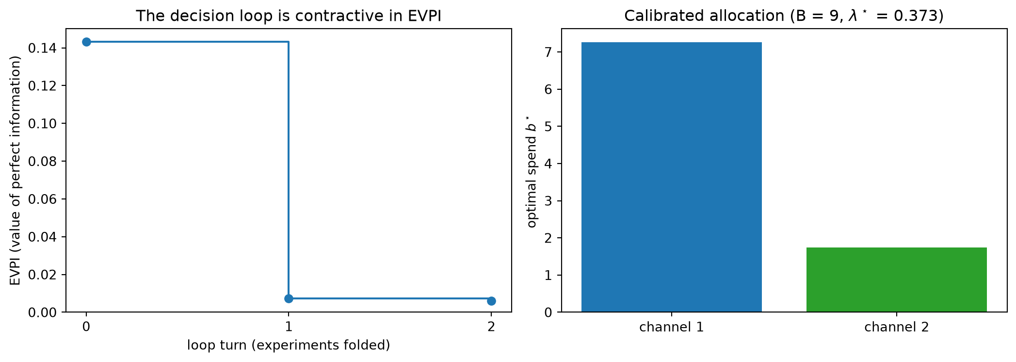
# The next experiment resolves the now-dominant direction; fold it and re-measure.v = np.array([1.0, 1.0]) # the remaining (total-effect) directiona_hat2, Ca2 = fold_lift(a_hat1, Ca1, v, s=0.10)evpi2 = evpi_from_posterior(a_hat2, Ca2)staircase = [evpi0, evpi1, evpi2]print("CLOSING THE LOOP")print(f" EVPI staircase across loop turns: "f"{evpi0:.4f} -> {evpi1:.4f} -> {evpi2:.4f}")assert evpi2 <= evpi1 +1e-9# monotone, turn after turn# --- Summary figure: the EVPI staircase, and the budget it justifies ---fig, ax = plt.subplots(1, 2, figsize=(11, 4))ax[0].step(range(len(staircase)), staircase, where="post", marker="o", color="tab:blue")ax[0].set_xticks(range(len(staircase)))ax[0].set_xlabel("loop turn (experiments folded)")ax[0].set_ylabel("EVPI (value of perfect information)")ax[0].set_title("The decision loop is contractive in EVPI")ax[0].set_ylim(0, None)ax[1].bar(["channel 1", "channel 2"], b_star, color=["tab:blue", "tab:green"])ax[1].set_ylabel("optimal spend $b^\\star$")ax[1].set_title(f"Calibrated allocation (B = {B:.0f}, $\\lambda^\\star$ = {lam[0]:.3f})")fig.tight_layout()plt.show()print("\nThe loop closed: data became a trustworthy budget, and named its next experiment.")
CLOSING THE LOOP
  EVPI staircase across loop turns: 0.1432 -> 0.0072 -> 0.0060
The loop closed: data became a trustworthy budget, and named its next experiment.
27.4 Exercises
27.4.1 C – Conceptual / Reading Comprehension
Walk the pipeline in words: state, for each of the six stages, what it receives from the stage before it and what it hands to the stage after. Where in the loop does raw data first become a decision, and where does the decision first become trustworthy?
The optimizer recommends moving 30% of the budget into search. Name two distinct things that would make you not trust that recommendation, and for each, name the stage of the pipeline that would have caught it.
Why does the EVPI fall monotonically as experiments are folded in, and what does that monotonicity guarantee about the loop as a whole? Could a single experiment ever make the decision worse?
The chapter proves no new theorems yet asserts several invariants in code. Where does the authority of those assertions come from — what makes them more than spot checks?
27.4.2 B – By Hand
A two-channel posterior has shadow price \lambda^\star = 0.37 shared across channels and remaining posterior standard deviations (0.45, 0.12) along two orthogonal directions. Which direction should the next experiment measure, and why?
The current EVPI is 0.14. A planned lift test will add precision 1/s^2 with s = 0.1 along the dominant uncertainty direction whose current standard deviation is 0.45. Qualitatively, will the post-experiment EVPI be closer to 0.14 or to 0? Justify from how a fold reshapes the posterior.
27.4.3 P – Prove It
Using the result of Chapter 22 (folding an experiment adds a positive-semidefinite precision term, so the posterior covariance decreases in the Loewner order), argue that the EVPI of the allocation decision is non-increasing under any fold. No new proof is required — state the chain of implications from “covariance decreases” to “EVPI does not increase.”
27.4.4 A – Applied / Code
Add a third channel to the data-generating process (with its own true coefficient and adstock rate) and rerun the entire pipeline. Report how the conditioning, the EVPI, and the optimal allocation change.
Vary the lift-test precision in Stage 4 (sweep s from 0.05 to 0.5) and trace how the post-calibration EVPI and the optimal split move. At what measurement noise does the experiment stop being worth running?
Replace the Stage 6 metamorphic invariant with a different one from Chapter 26 — for example permutation-invariance of the order in which two experiments are folded — and confirm the assembled system still passes.
27.5 Summary
Key concepts
The book is a single end-to-end pipeline: simulate (Ch.15) → fit (Ch.5/16) → check (Ch.11) → calibrate (Ch.19–22) → optimize (Ch.14/18) → test (Ch.23–26), each stage standing on a proved result.
A model that fits is not yet a decision that can be trusted; the EVPI (Ch.18) measures the gap and says when an experiment is worth running.
The prior store closes a decision loop: the optimizer’s shadow prices name the next experiment, whose result folds back and tightens the posterior.
Experiment selection is value-of-information decision theory — rank directions by their cost to the decision; the operational recipe is engineering, the principle is mathematics.
The book’s theorems serve double duty as the system’s specification and its tests.
Key takeaways
The loop is contractive in EVPI: each fold can only lower it (Ch.22), so the decision never gets worse by measuring more.
A budget decision is only as trustworthy as its least-identified direction — here, the spend/attribution contrast, the ridge that runs from Chapter 16 through Chapters 18 and 23.
Closed-form, deterministic components (the conjugate fit, the envelope-theorem shadow price) make the whole pipeline reproducible and testable end to end.
This is where the book lands: not a single model but a system — one that turns data into a budget, knows how much to trust it, and names what to measure next. Every chapter was one arc of that loop. Where to go next is to run it on your own data: swap the synthetic data-generating process for a real one, replace the closed-form fit with the sampler when the model outgrows conjugacy, and let the shadow prices choose your next experiment. The mathematics is in place; the engineering is yours.