Theory & Proofs
The four rungs below climb from the raw statement of Bayes’ theorem to the full Gaussian posterior for linear regression, each rung the clean warm-up for the next. The through-line, already glimpsed at the end of Chapter 4, is that ridge regression is the posterior mode; this chapter delivers the entire posterior that mode sat on top of.
Rung 1 — The Bayesian framework
The Bayesian framework reverses the direction of statistical inquiry. Chapter 4 asked which value of \beta maximizes p(y \mid \beta); Bayesian inference asks for the full conditional distribution p(\beta \mid y). The two ingredients are the prior p(\beta), encoding beliefs about \beta before any data arrive, and the likelihood p(y \mid \beta), scoring how probable the observed data would be under each candidate \beta. From the regression model y = X\beta + \varepsilon with \varepsilon \sim \mathcal{N}(0, \sigma^2 I) established in Chapter 3, the likelihood is
p(y \mid \beta) = (2\pi\sigma^2)^{-n/2}\exp\!\left(-\frac{1}{2\sigma^2}\lVert y - X\beta \rVert^2\right).
Bayes’ theorem (Chapter 3) combines prior and likelihood into the posterior:
p(\beta \mid y) = \frac{p(y \mid \beta)\, p(\beta)}{p(y)} \propto p(y \mid \beta)\, p(\beta).
The denominator p(y) = \int p(y \mid \beta)\, p(\beta)\, d\beta is the evidence — the prior-weighted probability of the data integrated over all \beta. It depends only on the model specification, not on \beta itself, and acts purely as the normalizing constant ensuring \int p(\beta \mid y)\, d\beta = 1. In the conjugate settings of rungs 2–4 we identify the posterior’s family by recognizing its kernel (the \beta-dependent factor in p(y \mid \beta)\, p(\beta)), after which the normalizing constant is forced by the known form of that family.
Alongside the posterior sits the posterior predictive distribution for a future observation \tilde{y}:
p(\tilde{y} \mid y) = \int p(\tilde{y} \mid \beta)\, p(\beta \mid y)\, d\beta.
This marginalizes over the full posterior uncertainty in \beta, producing a forecast that honestly propagates everything the data constrain and everything they do not. Chapter 4’s plug-in prediction \hat{y} = X\hat\beta_{\text{ridge}} treats \beta as fixed at its MAP estimate and discards the surrounding distribution entirely; the posterior predictive does not.
The unifying slogan is estimation becomes conditioning. We do not minimize an objective; we condition a probability model on the observed data. The posterior p(\beta \mid y) is the complete inferential object, and point estimates — posterior mode (MAP), posterior mean — are derived summaries of it. Chapter 4’s ridge estimator (X^\top X + \lambda I)^{-1}X^\top y is the MAP of p(\beta \mid y) under the prior \beta \sim \mathcal{N}(0, \tau^2 I): a single number extracted from a distribution whose full shape this chapter now develops.
Rung 2 — Conjugacy and the Beta–Binomial
When the evidence integral p(y) = \int p(y \mid \theta)\, p(\theta)\, d\theta admits a closed form, the posterior update reduces to algebra. A conjugate prior makes this systematic.
Definition. A prior family \mathcal{F} is conjugate to the likelihood p(y \mid \theta) if, whenever the prior p(\theta) \in \mathcal{F}, the posterior p(\theta \mid y) \in \mathcal{F} as well. The posterior remains in the same parametric family; observing data only updates the parameters.
The simplest MMM instance is channel-conversion attribution: does a media channel drive purchases? Observe k conversions from n exposures. The probability of the observed count depends on the conversion rate \theta \in (0, 1) through the Binomial kernel
p(k \mid \theta) \propto \theta^k(1 - \theta)^{n-k}.
Place a Beta prior on \theta: \theta \sim \text{Beta}(\alpha, \beta), with density p(\theta) \propto \theta^{\alpha-1}(1-\theta)^{\beta-1}.
Theorem (Beta–Binomial conjugacy). Under p(k \mid \theta) \propto \theta^k(1-\theta)^{n-k} with prior \theta \sim \text{Beta}(\alpha, \beta), the posterior is \theta \mid k \sim \text{Beta}(\alpha + k,\; \beta + n - k).
Proof. Multiply prior and likelihood kernel-to-kernel:
p(\theta \mid k) \propto \theta^k(1-\theta)^{n-k}\cdot\theta^{\alpha-1}(1-\theta)^{\beta-1} = \theta^{(\alpha+k)-1}(1-\theta)^{(\beta+n-k)-1}.
This is the kernel of a \text{Beta}(\alpha+k,\; \beta+n-k) density. Because a probability density must integrate to one, the normalizing constant is uniquely determined: it must be B(\alpha+k,\, \beta+n-k)^{-1}, the reciprocal of the Beta function at the updated parameters. Therefore
p(\theta \mid k) = \frac{\theta^{(\alpha+k)-1}(1-\theta)^{(\beta+n-k)-1}}{B(\alpha+k,\, \beta+n-k)}.
\blacksquare
The proof strategy is kernel-matching: identify the \theta-dependent pattern in p(k \mid \theta)\, p(\theta), recognize the distributional family, and read off the normalizing constant from the family’s known form without performing the integral directly.
The prior parameters \alpha and \beta act as pseudo-counts — \alpha prior successes and \beta prior failures — contributed before any data arrive. Observing k successes in n trials increments the counts to \alpha + k and \beta + (n - k). The posterior mean conversion rate
\mathbb{E}[\theta \mid k] = \frac{\alpha + k}{\alpha + \beta + n}
is a precision-weighted blend of the prior mean \alpha/(\alpha+\beta) and the empirical rate k/n, with the data winning as n \to \infty. This one-dimensional conjugate proof is the clean warm-up; the same kernel-matching strategy, applied to the Gaussian exponential family’s quadratic exponent, drives the next two rungs.
Rung 3 — The Gaussian conjugate
The Gaussian family closes under conjugate updating because its log-density is quadratic in the parameter. Completing the square — grouping the quadratic, linear, and constant terms in the parameter separately — reads off the posterior mean and variance directly, without evaluating any normalizing integral. This scalar calculation is the exact blueprint for the multivariate regression proof of Rung 4.
Let the prior be \mu \sim \mathcal{N}(\mu_0, \tau^2) and observe n i.i.d. draws y_1, \ldots, y_n \mid \mu \sim \mathcal{N}(\mu, \sigma^2) with known noise variance \sigma^2. Write \bar{y} = n^{-1}\sum_{i=1}^n y_i for the sample mean.
Theorem (Gaussian conjugacy). Under the above model, the posterior is \mu \mid y \sim \mathcal{N}(\mu_{\text{post}}, \sigma_{\text{post}}^2) with posterior precision 1/\sigma_{\text{post}}^2 = 1/\tau^2 + n/\sigma^2 and posterior mean \mu_{\text{post}} = \sigma_{\text{post}}^2(\mu_0/\tau^2 + n\bar{y}/\sigma^2).
Proof. The log-posterior, up to additive constants free of \mu, combines log-prior and log-likelihood:
\log p(\mu \mid y) = -\frac{(\mu - \mu_0)^2}{2\tau^2} - \frac{n(\mu - \bar{y})^2}{2\sigma^2} + \text{const},
where we used the identity \sum_i(y_i - \mu)^2 = n(\mu - \bar{y})^2 + \sum_i(y_i - \bar{y})^2 and absorbed the last piece into the constant. Expanding each squared term and grouping by powers of \mu:
\log p(\mu \mid y) = -\frac{1}{2}\!\left(\frac{1}{\tau^2} + \frac{n}{\sigma^2}\right)\mu^2 + \left(\frac{\mu_0}{\tau^2} + \frac{n\bar{y}}{\sigma^2}\right)\mu + \text{const}.
Define the posterior precision \sigma_{\text{post}}^{-2} = \tau^{-2} + n\sigma^{-2}. The quadratic and linear terms complete to a perfect square:
-\frac{(\mu - \mu_{\text{post}})^2}{2\sigma_{\text{post}}^2} + \text{const},
where the linear coefficient pins the posterior mean: \mu_{\text{post}} = \sigma_{\text{post}}^2(\mu_0/\tau^2 + n\bar{y}/\sigma^2). A negative quadratic in \mu is the hallmark of a Gaussian log-density, so the posterior is \mathcal{N}(\mu_{\text{post}}, \sigma_{\text{post}}^2) with the stated parameters.
\blacksquare
Two readings are essential for what follows. First, precisions add:
\frac{1}{\sigma_{\text{post}}^2} = \frac{1}{\tau^2} + \frac{n}{\sigma^2}.
Each observation contributes precision 1/\sigma^2; n observations contribute n/\sigma^2; the prior precision 1/\tau^2 stacks on top. Second, the posterior mean is a precision-weighted average of the prior mean \mu_0 and the sample mean \bar{y}:
\mu_{\text{post}} = \frac{\tau^{-2}}{\tau^{-2} + n\sigma^{-2}}\,\mu_0 + \frac{n\sigma^{-2}}{\tau^{-2} + n\sigma^{-2}}\,\bar{y}.
The weights sum to one and are proportional to the respective precisions. As n \to \infty the data precision dominates and \mu_{\text{post}} \to \bar{y}, recovering the maximum-likelihood estimate; a vague prior (\tau^2 \to \infty) yields the same limit. This scalar proof is the complete blueprint; Rung 4 replaces the scalar precision \sigma_{\text{post}}^{-2} with the p \times p precision matrix \Sigma_{\text{post}}^{-1}.
Rung 4 — Bayesian linear regression
We now execute the completing-the-square strategy for the full regression model. Place the Gaussian prior \beta \sim \mathcal{N}(0, \tau^2 I) on \beta \in \mathbb{R}^p and combine it with the Chapter 3 Gaussian likelihood y \mid \beta \sim \mathcal{N}(X\beta, \sigma^2 I). Taking -2 times the log-posterior and dropping all terms free of \beta:
-2\log p(\beta \mid y) = \frac{1}{\sigma^2}(y - X\beta)^\top(y - X\beta) + \frac{1}{\tau^2}\beta^\top\beta + \text{const}.
This is quadratic in \beta — the multivariate signature of a Gaussian posterior — so the proof is: expand, collect, complete the square, read off precision and mean.
Theorem (Bayesian linear regression). (Hoff 2009) Under y \mid \beta \sim \mathcal{N}(X\beta, \sigma^2 I) with prior \beta \sim \mathcal{N}(0, \tau^2 I), the posterior is \beta \mid y \sim \mathcal{N}(\mu_{\text{post}}, \Sigma_{\text{post}}) with \Sigma_{\text{post}} = (X^\top X/\sigma^2 + I/\tau^2)^{-1}, \mu_{\text{post}} = \Sigma_{\text{post}}\, X^\top y/\sigma^2, and the keystone identity \mu_{\text{post}} = (X^\top X + \lambda I)^{-1}X^\top y with \lambda = \sigma^2/\tau^2 — the Chapter 4 ridge estimator.
Proof. Expand the fit term (y - X\beta)^\top(y - X\beta) = y^\top y - 2\beta^\top X^\top y + \beta^\top X^\top X\beta and collect only the \beta-dependent terms:
-2\log p(\beta \mid y) = \beta^\top\!\left(\frac{X^\top X}{\sigma^2} + \frac{I}{\tau^2}\right)\!\beta - \frac{2}{\sigma^2}\beta^\top X^\top y + \text{const}.
Write A = X^\top X/\sigma^2 + I/\tau^2 — symmetric positive definite, since I/\tau^2 ensures strict positive definiteness regardless of the rank of X — and b = X^\top y/\sigma^2. The expression is \beta^\top A\beta - 2\beta^\top b + \text{const}. Complete the square via the matrix identity
\beta^\top A\beta - 2\beta^\top b = (\beta - A^{-1}b)^\top A\,(\beta - A^{-1}b) - b^\top A^{-1}b;
the term b^\top A^{-1}b is free of \beta and folds into the constant. Therefore
-2\log p(\beta \mid y) = (\beta - A^{-1}b)^\top A\,(\beta - A^{-1}b) + \text{const},
which is the kernel of \mathcal{N}(A^{-1}b,\, A^{-1}). Reading off the parameters:
\Sigma_{\text{post}} = A^{-1} = \left(\frac{X^\top X}{\sigma^2} + \frac{I}{\tau^2}\right)^{-1}, \qquad \mu_{\text{post}} = A^{-1}b = \Sigma_{\text{post}}\,\frac{X^\top y}{\sigma^2}.
To identify \mu_{\text{post}} as the ridge estimator, factor \sigma^{-2} from A:
A = \frac{1}{\sigma^2}\!\left(X^\top X + \frac{\sigma^2}{\tau^2}I\right) = \frac{1}{\sigma^2}(X^\top X + \lambda I), \qquad \lambda = \frac{\sigma^2}{\tau^2}.
Substituting into \mu_{\text{post}} = A^{-1}\,X^\top y/\sigma^2:
\begin{aligned}
\mu_{\text{post}} &= \left[\frac{1}{\sigma^2}(X^\top X + \lambda I)\right]^{-1}\frac{X^\top y}{\sigma^2} && \text{(substitute $A$)} \\[4pt]
&= \sigma^2(X^\top X + \lambda I)^{-1}\cdot\frac{X^\top y}{\sigma^2} && \text{(factor out $\sigma^{-2}$)} \\[4pt]
&= (X^\top X + \lambda I)^{-1}X^\top y && \text{($\sigma^2$ cancels).}
\end{aligned}
\blacksquare
The payoff is the chapter’s central claim. Chapter 4’s ridge estimator (X^\top X + \lambda I)^{-1}X^\top y was derived as the MAP estimate — the mode of p(\beta \mid y). The theorem above shows that this mode sits atop a full Gaussian posterior \mathcal{N}(\mu_{\text{post}}, \Sigma_{\text{post}}). For a Gaussian distribution, mode and mean coincide, so \hat\beta_{\text{ridge}} = \mu_{\text{post}} exactly: Chapter 4 computed the center of this distribution without realizing it was a distribution’s center. The new object now in hand is \Sigma_{\text{post}}, the joint uncertainty over all p coefficients simultaneously. The posterior precision \Sigma_{\text{post}}^{-1} = X^\top X/\sigma^2 + I/\tau^2 is the multivariate echo of Rung 3’s “precisions add”: data precision X^\top X/\sigma^2 and prior precision I/\tau^2 combine additively, and as n grows \Sigma_{\text{post}} \to \sigma^2(X^\top X)^{-1}, the OLS sampling covariance of Chapter 4. The next rungs cash \Sigma_{\text{post}} out: it generates credible intervals — direct probability statements about where each \beta_j lies given this data, the honest answer to the Motivation’s question — and the posterior predictive covariance that quantifies uncertainty bands in the MMM sales forecasts that budget-planning decisions require.
Rung 5 — Credible intervals and posterior summaries
The posterior \beta \mid y \sim \mathcal{N}(\mu_{\text{post}}, \Sigma_{\text{post}}) is a full probability distribution over \beta, and the most immediately useful thing a distribution can do is assign probability to regions. A credible interval for coefficient \beta_j is any interval [a, b] satisfying P(\beta_j \in [a, b] \mid y) = 1 - \alpha. The canonical choice is the central 1 - \alpha interval, which places equal probability mass \alpha/2 in each tail. For the Gaussian marginal \beta_j \mid y \sim \mathcal{N}(\mu_{\text{post},j},\, [\Sigma_{\text{post}}]_{jj}), the central interval takes the explicit form
\mu_{\text{post},j} \pm z_{1-\alpha/2}\sqrt{[\Sigma_{\text{post}}]_{jj}},
where z_{1-\alpha/2} is the standard normal upper-tail quantile and [\Sigma_{\text{post}}]_{jj} is the j-th diagonal entry of the posterior covariance.
The interpretation is literal: given the observed data y and the prior p(\beta), the probability that \beta_j falls inside this interval is exactly 1 - \alpha. No qualification about repeated sampling, no implicit reference to a long-run procedure — just a direct probability statement about the parameter given what was actually observed.
That directness stands in sharp contrast to the frequentist confidence interval from Chapter 4. In the OLS sampling framework, \beta is a fixed unknown and the data are the random objects; the interval \hat\beta_j \pm z_{1-\alpha/2}\hat\sigma_j is itself random because \hat\beta_j and \hat\sigma_j vary across datasets. “Ninety-five percent confidence” describes the long-run behavior of the procedure: ninety-five percent of all intervals constructed by this rule, over repeated draws of y from the true model, would contain the fixed true \beta_j. It is a statement about the interval, not about the parameter. A specific realized interval either does or does not contain the true \beta_j; frequentist theory assigns no probability to which case holds for the particular interval in front of you. The Bayesian credible interval makes exactly that statement — but only because the prior converts \beta from a fixed unknown into a random quantity whose probability can be discussed. The confidence interval requires no such commitment; the credible interval requires it and is rewarded with the more natural language.
The posterior also supports several point summaries. The posterior mean \mu_{\text{post}} = \mathbb{E}[\beta \mid y] minimizes posterior expected squared error. The posterior median minimizes expected absolute error. The MAP mode maximizes p(\beta \mid y). For the symmetric Gaussian posterior of Rung 4, all three coincide at \mu_{\text{post}} — which is precisely why Chapter 4’s ridge estimator, derived as the MAP mode, is also the posterior mean and posterior median. Once the non-negativity constraint of Rung 7 truncates the posterior, symmetry is lost: the mode shifts toward zero, the mean sits above it, and the median lies between them. The choice of point summary then becomes a substantive modeling decision, not a matter of convenience.
Rung 6 — The posterior predictive distribution
Rungs 1–5 characterize uncertainty in the model parameters \beta. Marketing decisions, however, are about outcomes — specifically, the sales \tilde{y} that a planned media spend \tilde{x} would generate next quarter. The posterior predictive distribution p(\tilde{y} \mid y) carries the posterior uncertainty in \beta forward into a forecast by marginalizing \beta out of the joint distribution p(\tilde{y}, \beta \mid y). For Bayesian linear regression this marginalization yields a closed form.
Theorem (posterior predictive). Under the model of Rung 4, let \tilde{y} = \tilde{x}^\top\beta + \tilde{\varepsilon} for a fixed covariate vector \tilde{x} \in \mathbb{R}^p, with \tilde{\varepsilon} \sim \mathcal{N}(0, \sigma^2) independent of \beta \mid y. Then \tilde{y} \mid y \sim \mathcal{N}\!\left(\tilde{x}^\top\mu_{\text{post}},\;\tilde{x}^\top\Sigma_{\text{post}}\,\tilde{x} + \sigma^2\right).
Proof. Conditional on y, the posterior is \beta \mid y \sim \mathcal{N}(\mu_{\text{post}}, \Sigma_{\text{post}}). The linear form \tilde{x}^\top\beta is a scalar affine image of a Gaussian vector, so by the affine-image property:
\tilde{x}^\top\beta \mid y \;\sim\; \mathcal{N}\!\left(\tilde{x}^\top\mu_{\text{post}},\;\tilde{x}^\top\Sigma_{\text{post}}\,\tilde{x}\right).
Adding the independent noise \tilde{\varepsilon} \sim \mathcal{N}(0, \sigma^2) to \tilde{x}^\top\beta sums independent Gaussians — means add and variances add — giving
\tilde{y} \mid y \;=\; \tilde{x}^\top\beta + \tilde{\varepsilon} \;\sim\; \mathcal{N}\!\left(\tilde{x}^\top\mu_{\text{post}},\;\tilde{x}^\top\Sigma_{\text{post}}\,\tilde{x} + \sigma^2\right).
\blacksquare
The predictive variance decomposes into two structurally distinct contributions. The term \tilde{x}^\top\Sigma_{\text{post}}\,\tilde{x} is parameter uncertainty (epistemic): it measures how much the posterior spread in \beta — our remaining uncertainty about the true model coefficients — propagates into spread in the forecast through the planned spend vector \tilde{x}. As the training data accumulate, \Sigma_{\text{post}} \to \sigma^2(X^\top X)^{-1} \to 0, so this term shrinks: more data tighten the posterior and narrow the predictive band. The term \sigma^2 is irreducible noise (aleatoric): genuine randomness in next quarter’s sales that would remain even if \beta were perfectly known. No amount of additional historical data eliminates it.
The practical consequence for MMM is direct. Forecasting next quarter’s sales at a planned spend \tilde{x} with the plug-in estimate \tilde{x}^\top\hat\beta_{\text{ridge}} reports only the predictive mean; it silently treats \Sigma_{\text{post}} = 0 and discards the parameter uncertainty entirely. Budget-planning decisions that depend on a risk margin — holding reserves when forecast uncertainty is wide, committing aggressively when the posterior is tight — cannot be made rationally from a point forecast alone. The posterior predictive distribution is the correct object for those decisions.
Rung 7 — Priors in practice and the conjugacy wall
The Gaussian prior \beta \sim \mathcal{N}(0, \tau^2 I) was mathematically convenient: it is conjugate to the Gaussian likelihood and yields the clean closed-form posterior of Rung 4. But the choice of \tau^2 is a genuine modeling decision, not a formality, and the conjugate Gaussian family covers only a small corner of the space of priors that real MMM problems require.
Prior calibration. The prior precision 1/\tau^2 is a dial controlling how strongly the prior pulls coefficients toward zero. Set \tau^2 large — a vague, diffuse prior — and the prior contributes negligible precision: \Sigma_{\text{post}}^{-1} \approx X^\top X/\sigma^2 and \mu_{\text{post}} \approx (X^\top X)^{-1}X^\top y, recovering OLS as \lambda = \sigma^2/\tau^2 \to 0. Set \tau^2 small — a tight, informative prior — and the coefficients are shrunk hard toward zero, corresponding to large-penalty ridge. The pseudo-count reading of Rung 2 generalizes: specifying a prior is equivalent to augmenting the dataset with imaginary observations encoding the prior beliefs. Weakly-informative defaults — Gaussian priors wide enough not to exclude plausible values but tight enough to prevent coefficients from drifting to implausible extremes — regularize without asserting strong substantive beliefs, and are now standard practice in applied Bayesian modeling (Gelman et al. 2013).
The MMM-critical sign constraint. Media channels are expected to drive sales, not suppress them: economic theory and advertising practice both demand \beta_j \ge 0 for each channel j. The natural encoding is a half-normal or truncated-normal prior on each channel coefficient:
p(\beta_j) \;\propto\; \exp\!\left(-\frac{\beta_j^2}{2\tau^2}\right)\mathbf{1}[\beta_j \ge 0].
This prior encodes the sign constraint directly, before any data arrive, rather than enforcing it by post-processing. But it is not conjugate to the Gaussian likelihood. Multiplying the Gaussian likelihood kernel by the truncated-Gaussian prior kernel produces a function that is Gaussian in shape but restricted to the non-negative half-line; the resulting posterior is a truncated normal with no closed-form expression for its mean vector or covariance matrix. Computing the posterior mean \mathbb{E}[\beta \mid y] now requires integrating over the truncated support, which involves the Gaussian CDF rather than elementary matrix algebra. Conjugacy was a luxury of the unconstrained Gaussian-Gaussian pairing; the indicator \mathbf{1}[\beta_j \ge 0] dissolves it.
The wall. The truncated-prior problem, though it forfeits conjugacy, is geometrically mild compared to what realistic MMM specifications introduce. Practical models pass media spend through an adstock (carryover) transformation — modeling the geometric decay of advertising’s lingering effect — and a saturation transformation — a diminishing-returns curve such as the Hill function f(x;\, K, n) = x^n/(K^n + x^n) — before the linear stage. Both transforms are nonlinear functions of their own parameters (decay rates, saturation half-points, Hill exponents), which means the full likelihood p(y \mid \beta, \theta_{\text{adstock}}, \theta_{\text{sat}}) is nonlinear in the model parameters. The negative log-posterior is no longer quadratic in all parameters simultaneously, the completing-the-square strategy of Rung 4 has no purchase, and the posterior p(\beta, \theta \mid y) has no closed form at all — not just for the covariance matrix, but for the entire distributional shape (Gelman et al. 2013). This is not a gap that more careful algebra might close. It is a structural barrier: the quadratic-exponent algebra that made Rung 4 tractable requires the log-likelihood to be quadratic in all parameters simultaneously, and nonlinear transforms break that condition permanently.
What follows from this barrier is not a dead end but a change of tools. A posterior that cannot be written down can still be sampled from, and samples from the posterior carry every inferential quantity that a closed-form expression would — posterior means, credible intervals, predictive distributions, and marginals over any subset of parameters. Constructing those samples is the business of Markov chain Monte Carlo, developed in Part III. Everything established in the rungs above — the prior, the likelihood, the Bayes’ theorem update, the posterior predictive decomposition of Rung 6 — defines exactly what MCMC will be sampling from. The conjugacy wall at the end of this section is not a flaw in the exposition; it is the precise structural reason that Part III is not optional.
Rung 8 — Eliciting priors: method of moments
Rung 7 argued that a prior is a genuine modeling choice; this rung makes that choice operational. In practice an analyst rarely thinks in hyperparameters — they think in business statements: “a coefficient around 0.3, but I am not very sure,” or “advertising’s effect roughly halves after three weeks.” The method of moments turns such a statement into hyperparameters by matching the prior’s mean and standard deviation to the elicited values and solving for the distribution’s parameters. Three workhorse families cover almost every MMM prior.
A bounded quantity — the Beta. A retention or decay fraction lives in (0,1), the natural support of \mathrm{Beta}(\alpha, \beta), whose mean and variance are \mu = \alpha/(\alpha+\beta) and \sigma^2 = \mu(1-\mu)/(\alpha+\beta+1). Writing the concentration \nu = \alpha + \beta, the variance identity inverts to
\nu = \frac{\mu(1-\mu)}{\sigma^2} - 1, \qquad \alpha = \mu\,\nu, \qquad \beta = (1-\mu)\,\nu,
valid exactly when \sigma^2 < \mu(1-\mu) — an elicited spread wider than a Bernoulli’s is infeasible and signals an overconfident or contradictory statement. This is precisely how an adstock retention prior is built: an elicited “half-life of three weeks” fixes a target mean retention \mu (geometric carryover \alpha^{t} reaches one-half at t = \ln 2 / \ln(1/\mu)), and a stated confidence fixes \sigma.
A positive quantity — the Gamma. For a strictly positive parameter such as a saturation half-point or a scale, \mathrm{Gamma}(\alpha, \beta) (shape–rate) has mean \alpha/\beta and variance \alpha/\beta^2, so matching \mu and \sigma gives
\alpha = \left(\frac{\mu}{\sigma}\right)^2, \qquad \beta = \frac{\mu}{\sigma^2}.
A positive quantity from a single number — the half-normal. When only a typical magnitude is offered and the quantity must stay non-negative, the half-normal of the previous section has the single parameter \sigma and mean \sigma\sqrt{2/\pi}, so a target mean \mu inverts to
\sigma = \mu\sqrt{\pi/2}.
The discipline these formulas enforce is twofold. First, check feasibility — the Beta bound above is a real constraint, not a formality. Second, mind the direction of the inversion: it is easy to confuse a half-life with a decay rate, or a mean with a mode, and a prior built from an inverted relationship is silently wrong — it samples cleanly and fits without complaint while encoding the opposite of the elicited belief. Verifying an elicited prior by drawing from it and inspecting the implied quantities (a prior predictive check, Rung 6) is the cheap insurance against exactly this failure, and we make it a routine step in Part V.
Worked Examples
Example (a) — Beta–Binomial by hand
A media buyer wants to estimate the conversion rate \theta of a new display campaign — the fraction of served impressions that result in a purchase. Before the campaign runs, domain knowledge suggests the rate is somewhere in the middle range (not extremely high, not near zero), and that belief carries mild weight. We encode it as a symmetric prior with mean 0.5:
\theta \sim \text{Beta}(2, 2).
The prior parameters are \alpha = 2 and \beta = 2, which act as pseudo-counts (Rung 2): two prior successes and two prior failures, as if we had already observed four imaginary exposures.
The data. Run the campaign for a day and observe k = 8 conversions in n = 10 exposures.
The posterior update. By the Beta–Binomial conjugacy theorem (Rung 2), the posterior is obtained by adding the observed counts to the prior pseudo-counts:
\theta \mid k \sim \text{Beta}(\alpha + k,\; \beta + n - k) = \text{Beta}(2 + 8,\; 2 + 2) = \text{Beta}(10, 4).
The arithmetic is kernel-matching in one line: the likelihood kernel \theta^k(1-\theta)^{n-k} = \theta^8(1-\theta)^2 multiplied by the prior kernel \theta^{\alpha-1}(1-\theta)^{\beta-1} = \theta^1(1-\theta)^1 yields \theta^9(1-\theta)^3, which is exactly the kernel of a \text{Beta}(10, 4) density. No integration required — recognizing the family forces the normalizing constant.
The posterior mean. The posterior mean (Rung 2) is
\mathbb{E}[\theta \mid k] = \frac{\alpha + k}{\alpha + \beta + n} = \frac{2 + 8}{2 + 2 + 10} = \frac{10}{14} \approx 0.714.
Comparing the three summaries side by side makes the structure vivid:
\underbrace{0.500}_{\text{prior mean}} \quad < \quad \underbrace{0.714}_{\text{posterior mean}} \quad < \quad \underbrace{0.800}_{\text{MLE}\; k/n}.
The MLE \hat\theta = 8/10 = 0.800 is the value that maximizes the likelihood alone, giving full weight to the observed data and none to prior belief. The posterior mean is pulled from 0.800 toward 0.500 — this is shrinkage, driven by the prior pseudo-count total \alpha + \beta = 4 in competition with the real data count n = 10.
Interpretation and shrinkage mechanics. The four prior pseudo-observations carry 4/(4 + 10) \approx 29\% of the total evidential weight, so their pull is visible but not dominant. Had the campaign run for n = 100 exposures (say, 80 conversions), the posterior mean would be (2 + 80)/(4 + 100) \approx 0.788, much closer to the empirical rate 0.800. The prior’s influence fades as real data accumulate — not discarded, simply outweighed. This is the quantitative expression of the Rung 3 formula: the posterior mean is a precision-weighted blend of prior and data, with the data’s precision growing with n while the prior’s precision stays fixed.
The posterior \text{Beta}(10, 4) is also sharper than the prior \text{Beta}(2, 2). Prior variance is \alpha\beta/((\alpha+\beta)^2(\alpha+\beta+1)) = 4/(16\cdot 5) = 0.050; posterior variance is 10\cdot 4/(14^2\cdot 15) \approx 0.014, a reduction by more than a factor of three. The data added information and the posterior reflects it — the distribution has contracted around the updated belief.
Example (b) — Bayesian linear regression by hand
We revisit the exact dataset from Chapter 4’s first worked example: four weeks of a single media channel with intercept,
X = \begin{bmatrix} 1 & 1 \\ 1 & 2 \\ 1 & 3 \\ 1 & 4 \end{bmatrix}, \qquad y = \begin{bmatrix} 2 \\ 2 \\ 4 \\ 5 \end{bmatrix},
now treated within the Bayesian framework. We take the noise variance known at \sigma^2 = 1 and place a zero-mean Gaussian prior \beta \sim \mathcal{N}(0, \tau^2 I) with \tau^2 = 1. The penalty ratio is \lambda = \sigma^2/\tau^2 = 1. With both variances equal to one, the posterior formulas of Rung 4 simplify cleanly: the posterior covariance is (X^\top X + I)^{-1} and the posterior mean is (X^\top X + I)^{-1} X^\top y — exactly the ridge estimator at \lambda = 1.
The ingredients. The cross-product matrix and vector are identical to Chapter 4:
X^\top X = \begin{bmatrix} 4 & 10 \\ 10 & 30 \end{bmatrix}, \qquad X^\top y = \begin{bmatrix} 13 \\ 38 \end{bmatrix}.
The posterior covariance. Add I to X^\top X:
X^\top X + I = \begin{bmatrix} 4+1 & 10 \\ 10 & 30+1 \end{bmatrix} = \begin{bmatrix} 5 & 10 \\ 10 & 31 \end{bmatrix}.
The determinant is 5 \cdot 31 - 10 \cdot 10 = 155 - 100 = 55. Applying the 2 \times 2 inversion rule (swap the diagonal entries, negate the off-diagonal entries, divide by the determinant):
\Sigma_{\text{post}} = \frac{1}{55}\begin{bmatrix} 31 & -10 \\ -10 & 5 \end{bmatrix} = \begin{bmatrix} 0.5636 & -0.1818 \\ -0.1818 & 0.0909 \end{bmatrix}.
The diagonal entries are the posterior variances: 0.5636 for the intercept \beta_0 and 0.0909 for the slope \beta_1. The negative off-diagonal entry reflects that, conditional on the data, uncertainty in the intercept and slope are negatively correlated — a higher-than-expected intercept implies a lower-than-expected slope.
The posterior mean. Apply \mu_{\text{post}} = \Sigma_{\text{post}}\, X^\top y:
\mu_{\text{post}} = \frac{1}{55}\begin{bmatrix} 31 & -10 \\ -10 & 5 \end{bmatrix}\begin{bmatrix} 13 \\ 38 \end{bmatrix} = \frac{1}{55}\begin{bmatrix} 31\cdot 13 - 10\cdot 38 \\ -10\cdot 13 + 5\cdot 38 \end{bmatrix}.
Computing entry by entry: 31\cdot 13 = 403 and 10\cdot 38 = 380, so the first entry is 403 - 380 = 23; 10\cdot 13 = 130 and 5\cdot 38 = 190, so the second entry is -130 + 190 = 60. Therefore
\mu_{\text{post}} = \frac{1}{55}\begin{bmatrix} 23 \\ 60 \end{bmatrix} = \begin{bmatrix} 0.4182 \\ 1.0909 \end{bmatrix}.
The posterior mean intercept is 0.4182 and the posterior mean slope is 1.0909.
The ridge connection confirmed. By construction, \mu_{\text{post}} = (X^\top X + \lambda I)^{-1}X^\top y with \lambda = 1: this is precisely the ridge estimator Chapter 4 derived as the MAP estimate. The theorem of Rung 4 guarantees the two are the same object — Chapter 4 extracted the mode of a distribution whose full shape we now hold. Chapter 4’s OLS slope was \hat\beta_1 = 1.1; the posterior mean slope 1.0909 is slightly smaller, pulled toward zero by the prior precision I/\tau^2 = I. That pull is the same ridge shrinkage Chapter 4 described as a penalty, now understood as the posterior mean of a Gaussian prior centered at zero.
The 95% credible interval for the slope. The posterior marginal for the slope (Rung 5) is
\beta_1 \mid y \;\sim\; \mathcal{N}\!\left(1.0909,\; 0.0909\right),
reading \mu_{\text{post},1} = 1.0909 and [\Sigma_{\text{post}}]_{11} = 0.0909 from the results above. The posterior standard deviation is \sqrt{0.0909} = 0.3015. The central 95% credible interval is
1.0909 \pm 1.96 \times 0.3015 = 1.0909 \pm 0.5910 = [0.500,\; 1.682].
This is a direct probability statement: given the observed data y and the prior \mathcal{N}(0, I), the probability that the true slope lies in [0.500, 1.682] is 0.95.
Contrast with Chapter 4’s confidence interval. Chapter 4 computed the OLS 95% confidence interval for the slope on this same data as
1.1 \pm 4.303 \times 0.2646 = 1.1 \pm 1.138 = [-0.038,\; 2.238],
using the Student-t quantile t_{2,\,0.975} = 4.303 for n - p = 2 degrees of freedom (an extremely wide quantile for only two degrees of freedom). The Bayesian 95% credible interval [0.500, 1.682] is substantially narrower: width 1.182 versus the frequentist width 2.276, a factor of nearly two. Two forces drive the gap. First, the prior \mathcal{N}(0, \tau^2 I) contributed extra precision I/\tau^2 = I to the posterior precision matrix \Sigma_{\text{post}}^{-1} = X^\top X + I — information the frequentist analysis had no access to. Second, the Bayesian interval uses the standard normal quantile z_{0.975} = 1.96 because \sigma^2 is treated as known, whereas frequentist inference must account for the additional uncertainty in estimating \sigma^2 from only two residual degrees of freedom, inflating the quantile from 1.96 to 4.303. Together these effects compress the credible interval substantially on both ends. The Bayesian interval also carries the more natural interpretation: not a statement about a long-run procedure, but a direct claim that the posterior places 95\% of its mass on \beta_1 \in [0.500, 1.682] given this data and this prior.
Exercises
C – Conceptual / Reading Comprehension
C1. For the Bayesian linear regression model of Rung 4, Bayes’ theorem delivers the posterior p(\beta \mid y) \propto p(y \mid \beta)\,p(\beta) over the full coefficient vector \beta \in \mathbb{R}^p. The ridge MAP estimator \hat\beta_{\text{ridge}} = (X^\top X + \lambda I)^{-1}X^\top y extracts the mode of this distribution; since the Rung 4 posterior is Gaussian, its mode, mean, and median all coincide. Explain precisely why p(\beta \mid y) — the entire distribution — is “the whole inferential object,” whereas the single number \hat\beta_{\text{TV}} = 1.8 is merely a scalar derived from that object: what information does the marginal posterior p(\beta_{\text{TV}} \mid y) contain that \hat\beta_{\text{TV}} = 1.8 discards? Then explain what additional question the posterior predictive distribution
p(\tilde y \mid y) = \int p(\tilde y \mid \beta)\,p(\beta \mid y)\,d\beta
answers that p(\beta \mid y) alone cannot. Specifically: why does a marketing analyst planning next quarter’s budget at planned spend \tilde x need p(\tilde y \mid y) rather than just p(\beta \mid y), and what two structurally distinct components make up the predictive variance \tilde x^\top \Sigma_{\text{post}}\,\tilde x + \sigma^2 — which shrinks with more data and which does not?
C2. A Bayesian analyst fits a media-mix model and reports the 95% credible interval \beta_{\text{TV}} \in [0.5,\,1.7] for the TV spend coefficient. State precisely what this interval claims: write out the formal probability statement it makes, identify what is random and what is fixed in that statement, and name the object — prior, likelihood, or posterior — that licenses it. Then contrast it with the frequentist 95% confidence interval for \beta_{\text{TV}}: in the sampling-distribution framework of Chapter 4, \beta is a fixed unknown and \hat\beta_{\text{TV}} is the random object, so the 95% refers to a long-run property of the procedure over hypothetical repeated datasets. Explain why, for a specific realized confidence interval, the frequentist framework assigns no probability to the claim “the true \beta_{\text{TV}} lies in this interval” — and why the Bayesian credible interval makes exactly that claim without contradiction. Conclude by naming the one assumption the credible-interval statement requires that the confidence-interval statement does not, and argue in one sentence why, in practice, an MMM analyst almost always possesses prior knowledge (sign constraints, order-of-magnitude channel benchmarks) that makes this assumption a modeling feature rather than an arbitrary imposition.
C3. The closed-form Gaussian posterior of Rung 4 relies on the prior \beta_j \sim \mathcal{N}(0,\tau^2) being conjugate to the Gaussian likelihood. Suppose instead you impose the half-normal prior
p(\beta_j) \;\propto\; \exp\!\left(-\frac{\beta_j^2}{2\tau^2}\right)\mathbf{1}[\beta_j \ge 0]
on each media-channel coefficient \beta_j to enforce the economic constraint that advertising cannot suppress sales. Explain in detail why this prior destroys the closed-form posterior of Rung 4: what does multiplying the Gaussian likelihood kernel by the half-normal prior kernel produce, and why can the posterior mean \mathbb{E}[\beta_j \mid y] no longer be read off by completing the square? Identify the specific integral involving the Gaussian CDF that must now be evaluated numerically in place of elementary matrix algebra. Then explain how adstock (geometric carryover) and saturation transforms compound the problem: if media spend x_{jt} enters the likelihood through a nonlinear transformation f(x_{jt};\,\theta) — such as the Hill saturation function f(x;\,K,n) = x^n/(K^n + x^n) — with its own parameters \theta, what structural property of the log-posterior that made Rung 4’s completing-the-square strategy work is permanently lost, and why does that loss make Markov chain Monte Carlo (Part III) a mathematical necessity rather than a computational convenience?
B – By Hand
B1. A media analytics team wants to estimate the conversion rate \theta — the probability that a served impression results in a purchase — for a new paid-search campaign. Historical data from similar campaigns support a strong belief that high-intent search placements convert well, so the team encodes a prior that places substantial mass above 0.5: \theta \sim \text{Beta}(3,\,1), with prior mean \alpha/(\alpha+\beta) = 3/4 = 0.75. A one-week test produces k = 5 conversions from n = 8 served impressions. (a) Apply the Beta–Binomial conjugacy theorem of Rung 2: write out the kernel multiplication p(\theta \mid k) \propto \theta^k(1-\theta)^{n-k}\cdot\theta^{\alpha-1}(1-\theta)^{\beta-1}, collect exponents, and identify the posterior distribution by name and parameters. (b) Compute the posterior mean \mathbb{E}[\theta \mid k] = (\alpha+k)/(\alpha+\beta+n) numerically and verify it equals 2/3 \approx 0.667. (c) Compare the posterior mean to the MLE \hat\theta = k/n and the prior mean, display the three values on a number line, and explain in one sentence which direction the prior pulls the posterior mean relative to the MLE and why.
B2. A marketing data scientist models the mean weekly incremental sales lift \mu (in thousands of units) from a new channel’s first activation quarter. Before any data arrive she encodes the prior \mu \sim \mathcal{N}(\mu_0,\,\tau^2) with \mu_0 = 0 and \tau^2 = 4 — centered at zero with substantial spread — and treats the within-week noise variance as known: \sigma^2 = 9. She then observes n = 9 i.i.d. weekly lifts with sample mean \bar{y} = 6.0. Using the Gaussian conjugate update of Rung 3: (a) compute the posterior precision 1/\sigma_{\text{post}}^2 = 1/\tau^2 + n/\sigma^2 numerically, then invert to find \sigma_{\text{post}}^2; (b) compute the posterior mean \mu_{\text{post}} = \sigma_{\text{post}}^2(\mu_0/\tau^2 + n\bar{y}/\sigma^2) and verify it equals 4.8; (c) rewrite \mu_{\text{post}} as an explicit precision-weighted average of \mu_0 and \bar{y}, state the numerical weight attached to each, verify the weights sum to one, and explain in one sentence why \mu_{\text{post}} = 4.8 lies closer to \bar{y} = 6.0 than to \mu_0 = 0.
B3. A reduced MMM design for a two-channel campaign yields the cross-product matrix and moment vector
X^\top X = \begin{bmatrix} 4 & 2 \\ 2 & 4 \end{bmatrix}, \qquad X^\top y = \begin{bmatrix} 6 \\ 4 \end{bmatrix}.
The noise variance is known: \sigma^2 = 1. Place the Gaussian prior \beta \sim \mathcal{N}(0,\,\tau^2 I) with \tau^2 = 1/2, giving \lambda = \sigma^2/\tau^2 = 2. (a) Form X^\top X + \lambda I and compute its determinant. (b) Invert X^\top X + \lambda I explicitly using the 2\times2 inversion rule: swap the diagonal entries, negate the off-diagonal entries, divide by the determinant. (c) Multiply by X^\top y to obtain the posterior mean \mu_{\text{post}} = (X^\top X + \lambda I)^{-1}X^\top y and verify it equals (7/8,\; 3/8) = (0.875,\; 0.375). (d) Confirm that this is the ridge estimator of Chapter 4 at \lambda = 2 — the two calculations are identical — and state in one sentence what \Sigma_{\text{post}} = (X^\top X + \lambda I)^{-1} adds beyond the single point \mu_{\text{post}} that the ridge formula alone does not provide.
P – Prove It
P1. Prove that the Beta distribution is conjugate to the Binomial likelihood. Let k \mid \theta \sim \text{Binomial}(n,\theta) so the likelihood kernel is p(k \mid \theta) \propto \theta^k(1-\theta)^{n-k}, and let the prior be \theta \sim \text{Beta}(\alpha, \beta) with density proportional to \theta^{\alpha-1}(1-\theta)^{\beta-1} on (0,1). (a) Multiply the prior and likelihood kernels and collect exponents to identify the functional form of p(\theta \mid k); state the posterior distribution by name and parameters. (b) Explain in one or two sentences why recognizing the distributional family of the kernel is sufficient to determine the full posterior density — including its normalizing constant — without evaluating any integral. (c) Write the posterior mean as (\alpha+k)/(\alpha+\beta+n) and show algebraically that it is a convex combination of the prior mean \alpha/(\alpha+\beta) and the MLE k/n: find explicit non-negative weights w and 1-w (summing to one, depending on \alpha, \beta, n) such that (\alpha+k)/(\alpha+\beta+n) = w\cdot\alpha/(\alpha+\beta) + (1-w)\cdot k/n.
P2. Prove the Gaussian conjugate update of Rung 3. Let the prior be \mu \sim \mathcal{N}(\mu_0, \tau^2) and let y_1, \ldots, y_n \mid \mu be i.i.d. \mathcal{N}(\mu, \sigma^2) with \sigma^2 known; write \bar{y} = n^{-1}\sum_{i=1}^n y_i. (a) Use the identity \sum_{i=1}^n (y_i - \mu)^2 = n(\mu - \bar{y})^2 + \sum_{i=1}^n(y_i-\bar{y})^2 to write -2\log p(\mu \mid y) up to additive constants free of \mu, and show it equals
\left(\frac{1}{\tau^2} + \frac{n}{\sigma^2}\right)\mu^2 - 2\left(\frac{\mu_0}{\tau^2} + \frac{n\bar{y}}{\sigma^2}\right)\mu + \text{const}.
- Complete the square in \mu to write this as (\mu - \mu_{\text{post}})^2/\sigma_{\text{post}}^2 + \text{const}; read off the posterior precision \sigma_{\text{post}}^{-2} and the posterior mean \mu_{\text{post}} in terms of \mu_0, \tau^2, \bar{y}, \sigma^2, n. (c) Verify that \mu_{\text{post}} can be rewritten as the precision-weighted average
\mu_{\text{post}} = \frac{\tau^{-2}}{\tau^{-2} + n\sigma^{-2}}\,\mu_0 + \frac{n\sigma^{-2}}{\tau^{-2} + n\sigma^{-2}}\,\bar{y},
and confirm the two weights sum to one.
P3. Prove the Bayesian linear regression posterior of Rung 4, reproducing its derivation from scratch. Let the prior be \beta \sim \mathcal{N}(0, \tau^2 I) with \beta \in \mathbb{R}^p, and let y \mid \beta \sim \mathcal{N}(X\beta, \sigma^2 I) with X \in \mathbb{R}^{n \times p} fixed and \sigma^2 known. (a) Write -2\log p(\beta \mid y) up to constants free of \beta, expand (y - X\beta)^\top(y - X\beta), discard all \beta-free terms, and collect the remaining terms to exhibit the form \beta^\top A\beta - 2\beta^\top b + \text{const}; identify A and b explicitly, and justify why A is symmetric positive definite. (b) Apply the matrix completing-the-square identity
\beta^\top A\beta - 2\beta^\top b = (\beta - A^{-1}b)^\top A\,(\beta - A^{-1}b) - b^\top A^{-1}b
to conclude that \beta \mid y \sim \mathcal{N}(\mu_{\text{post}}, \Sigma_{\text{post}}) with \Sigma_{\text{post}} = A^{-1} and \mu_{\text{post}} = A^{-1}b; explain why identifying the distributional kernel forces the normalizing constant. (c) Factor A = (X^\top X + \lambda I)/\sigma^2 with \lambda = \sigma^2/\tau^2 and substitute into \mu_{\text{post}} = A^{-1}b to show \mu_{\text{post}} = (X^\top X + \lambda I)^{-1}X^\top y, confirming that the posterior mean equals the ridge estimator of Chapter 4 exactly.
A – Applied / Code
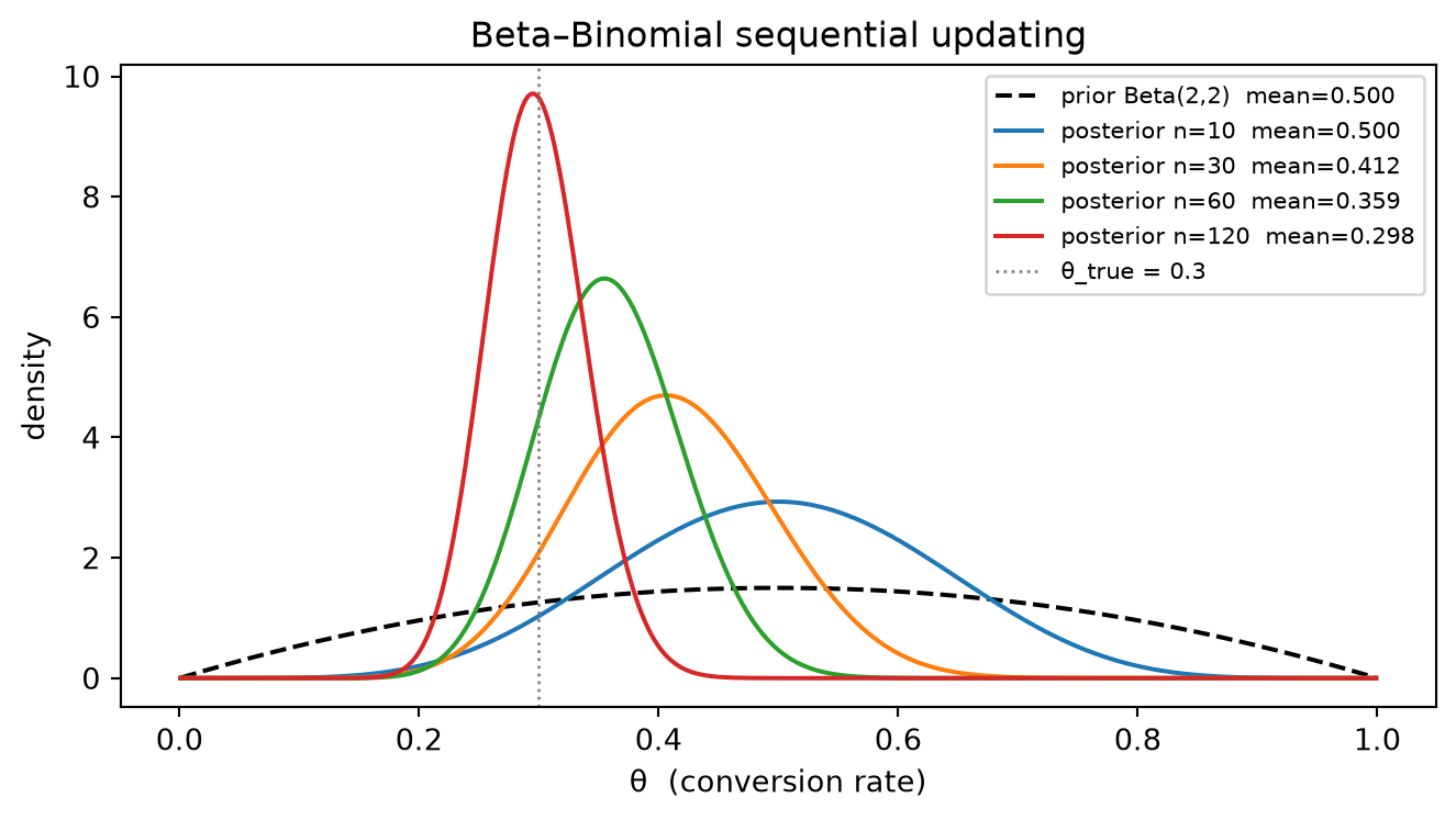
A1. Beta–Binomial sequential updating. A retargeting campaign has true conversion rate \theta_{\text{true}} = 0.40. Start from the prior \theta \sim \text{Beta}(2,\,8) (prior mean = 0.20, encoding a conservative baseline before retargeting optimization). Generate N = 200 i.i.d. Bernoulli(0.40) impressions using a fixed random seed. Process them in four sequential batches of sizes 10, 20, 70, and 100: after each batch apply the closed-form conjugate update (\alpha, \beta) \gets (\alpha + k_{\text{batch}},\; \beta + n_{\text{batch}} - k_{\text{batch}}) and record the posterior mean and the 95% central credible interval [\text{Beta.ppf}(0.025,\alpha,\beta),\;\text{Beta.ppf}(0.975,\alpha,\beta)]. Plot the prior density and the four posterior densities on a single axes over \theta \in (0,1), labeling each curve with its running sample size and posterior mean; overlay a vertical line at \theta_{\text{true}} = 0.40 to show the posterior sharpening toward the true rate as data accumulate. For the final posterior after all 200 observations, construct a numerical baseline: evaluate q(\theta_i) = \theta_i^{\alpha_0 + k_{\text{total}} - 1}(1-\theta_i)^{\beta_0 + (n_{\text{total}} - k_{\text{total}}) - 1} on a fine grid of 500 equally-spaced points \theta_i \in (0,1) (where \alpha_0 = 2, \beta_0 = 8), normalize so \sum_i q(\theta_i)\,\Delta\theta = 1, overlay on the closed-form \text{Beta}(\alpha_{\text{final}}, \beta_{\text{final}}) density, and verify that the two means agree to at least three significant figures.
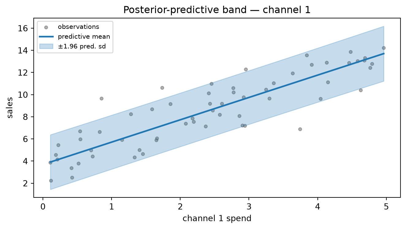
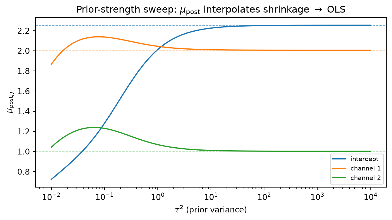
A2. Bayesian linear regression: posterior, predictive, and prior sweep. Simulate n = 80 observations from a two-channel MMM with intercept: build X \in \mathbb{R}^{80\times3} by stacking a column of ones with channel-1 spend drawn from \text{Uniform}(0,5) and channel-2 spend from \text{Uniform}(0,3); set \beta_{\text{true}} = [2.0,\;1.5,\;0.8]^\top and generate y = X\beta_{\text{true}} + \varepsilon with \varepsilon \sim \mathcal{N}(0,\,\sigma^2 I), \sigma^2 = 2.0. Fix \tau^2 = 5.0, giving \lambda = \sigma^2/\tau^2 = 0.4. Compute the closed-form posterior
\Sigma_{\text{post}} = \left(\frac{X^\top X}{\sigma^2} + \frac{I}{\tau^2}\right)^{-1}, \qquad \mu_{\text{post}} = \Sigma_{\text{post}}\,\frac{X^\top y}{\sigma^2},
and assert programmatically that \mu_{\text{post}} equals the ridge estimate (X^\top X + \lambda I)^{-1}X^\top y to machine precision. (a) Draw S = 10{,}000 posterior samples \beta^{(s)} \sim \mathcal{N}(\mu_{\text{post}},\Sigma_{\text{post}}) and report, for each coefficient j, the analytic 95% credible interval \mu_{\text{post},j} \pm 1.96\sqrt{[\Sigma_{\text{post}}]_{jj}} alongside the empirical 2.5th and 97.5th percentiles of the samples; confirm the two sets of bounds agree to two decimal places. (b) Sweep channel-1 spend over 100 equally-spaced grid points in [0,5] while holding channel-2 spend at its training-set mean; at each grid point \tilde x, compute the predictive mean \tilde x^\top\mu_{\text{post}} and predictive standard deviation \sqrt{\tilde x^\top\Sigma_{\text{post}}\,\tilde x + \sigma^2}; plot the mean curve with a \pm 1.96 predictive band alongside the training scatter. (c) Sweep \tau^2 over 60 log-spaced values from 10^{-2} to 10^4; at each value recompute \mu_{\text{post}} and plot all three coefficient traces as a function of \tau^2 on a log-x-axis, overlaying the OLS solution (X^\top X)^{-1}X^\top y as horizontal dashed lines; confirm that the traces converge to OLS as \tau^2 \to \infty and collapse toward zero as \tau^2 \to 0.