Motivation
Chapter 5 derived the full Bayesian posterior for a single regression: place a prior \beta \sim \mathcal{N}(0, \tau^2 I) on a coefficient vector, observe one dataset, and the posterior is a Gaussian whose mean is the ridge estimator and whose covariance quantifies all remaining uncertainty. That story is complete and exact — for a national campaign. Practitioners running MMM across the approximately fifty U.S. designated market areas confront a decision that shatters the single-population model at the outset. The recurring model for this chapter is
y_g = X_g\beta_g + \varepsilon_g, \qquad \varepsilon_g \sim \mathcal{N}(0,\sigma^2 I),
where y_g \in \mathbb{R}^{T} is the vector of weekly sales in geography g, X_g \in \mathbb{R}^{T \times p} is its media-spend design matrix, and \beta_g \in \mathbb{R}^p is allowed to vary across geographies. The choice is between two obviously inadequate extremes. Complete pooling fits one national model with a single shared \beta, asserting that TV’s incremental return is the same in Chicago and rural Nebraska and that every geography runs on the same data-generating process. This is convenient and almost certainly wrong: the bias from forcing a common slope across genuinely heterogeneous markets distorts every coefficient, and the one it distorts most is usually the channel coefficient the analyst needs most to trust. No pooling fits fifty independent regressions, each confined to its own slice of data. A dense metro with years of weekly observations yields a tolerable per-geo estimate; a small DMA with a handful of active weeks produces an OLS estimate that is effectively pure sampling noise — a diffuse Bayesian prior on the per-geo fit does nothing to improve matters because the local likelihood is too weak to constrain the posterior away from its baseline.
“Des Moines came back with a TV coefficient of 9.2 — absurd on 10 weeks of data. Do you trust it, throw it out, or shrink it toward the national average — and by exactly how much?”
The answer is partial pooling — the principled middle ground — and it is delivered by modeling the per-geo coefficients as draws from a shared population distribution, \beta_g \sim \mathcal{N}(\mu, \tau^2 I). This single hierarchical prior converts fifty isolated estimation problems into one joint model whose posterior borrows strength across all geographies simultaneously: coefficient estimates for data-rich geographies converge toward their local OLS solutions while estimates for data-sparse geographies are shrunk toward the population mean \mu, by exactly the amount the joint evidence supports.
The shrinkage is not a heuristic — it is the posterior mean of the multilevel model, and it falls straight out of Chapter 5’s “precisions add” rule operating one level up: the within-geography data precision n_g/\sigma^2 is weighed against the between-geography precision 1/\tau^2, and their ratio determines exactly how hard each geography is pulled toward the national mean.
This chapter delivers four payoffs from that mechanism. The shrinkage formula — the closed-form posterior mean for each \beta_g as a function of its local data and the population parameters — is the keystone result. The James–Stein theorem provides a finite-sample guarantee: any estimator that shrinks per-group estimates toward a common center has strictly lower total squared error than the collection of unpooled per-group fits, a dominance result that holds regardless of the true \mu and \tau^2. The between-geography variance \tau^2 is estimated from all the geographies at once rather than chosen by the analyst, so the degree of pooling is a property the data determine rather than an assumption imposed on them.
And because the joint posterior over all \beta_g, \mu, and \tau^2 is non-conjugate — marginalizing over \tau^2 does not yield a closed form — the chapter closes with the Gibbs sampler whose conjugate full conditionals are each a Gaussian-on-Gaussian update identical to a Chapter 5 result. That Gibbs sampler is the direct prototype for the Markov chain Monte Carlo methods of Part III, and the conjugacy wall it meets is precisely the structural reason Part III is not optional.
Theory & Proofs
The three rungs below build the pooling taxonomy, derive the closed-form shrinkage formula, and establish the frequentist guarantee that makes pooling universally preferable to unpooled estimation. The through-line: complete pooling and no pooling are the degenerate limits of one hierarchical model; partial pooling is Chapter 5’s “precisions add” rule operating one level up, across groups rather than within them; and James–Stein proves that shrinking toward any common center strictly lowers total squared error for every possible configuration of true group effects.
Rung 1 — Three stances: complete, no, and partial pooling
To fix ideas, work with a scalar per-geography parameter. Let \theta_g be a single channel’s effect in geography g, for g = 1, \ldots, G. Each geography contributes n_g observations with known noise variance \sigma^2, so the sufficient statistic is the group sample mean \bar y_g, distributed as
\bar y_g \mid \theta_g \;\sim\; \mathcal{N}\!\left(\theta_g,\; \frac{\sigma^2}{n_g}\right).
The hierarchical prior on the true group effects is
\theta_g \;\sim\; \mathcal{N}(\mu,\, \tau^2),
with \mu the population mean and \tau^2 the between-geography variance. This two-level structure encompasses three distinct stances depending on \tau^2.
Complete pooling is the limit \tau^2 \to 0. As \tau^2 shrinks to zero the prior concentrates at \mu, forcing every group effect to the single shared value \theta_g = \mu. A national MMM model that fits one TV coefficient across all fifty DMAs operates under complete pooling: one estimate, low variance, but systematically biased whenever geographies genuinely differ.
No pooling is the limit \tau^2 \to \infty. As \tau^2 \to \infty the prior flattens to uninformative, so each group is estimated in isolation: the posterior mean collapses to the group sample mean \hat\theta_g = \bar y_g. Fitting fifty independent regressions, each confined to its own DMA, is the no-pooling extreme. There is no bias from misspecified homogeneity, but for small-n_g geographies the sample mean \bar y_g has sampling variance \sigma^2/n_g that grows without bound as n_g shrinks.
Partial pooling occupies the interior: 0 < \tau^2 < \infty. The prior is informative enough to draw group estimates toward the population mean, but not so tight that it erases genuine group differences. Each geography’s shrinkage weight adjusts in proportion to how much local data it provides, and that weight is what the rest of this section derives.
The tension between the two extremes is exactly Chapter 4’s bias–variance decomposition of the mean-squared error. For any estimator \hat\theta_g,
\mathbb{E}[(\hat\theta_g - \theta_g)^2] \;=\; \bigl(\mathbb{E}[\hat\theta_g] - \theta_g\bigr)^2 + \operatorname{Var}(\hat\theta_g).
Complete pooling minimizes variance at the cost of bias squared; no pooling eliminates bias at the cost of variance. Rung 2 delivers the estimator that balances the two, per geography, and its shrinkage weight \lambda_g is the precise quantitative answer to the Motivation’s “by exactly how much?”
Rung 2 — Partial pooling as precision-weighted shrinkage
The Gaussian two-level model of Rung 1 is exactly the Gaussian conjugate setup of Chapter 5 Rung 3, applied separately to each group. The likelihood \bar y_g \mid \theta_g \sim \mathcal{N}(\theta_g, \sigma^2/n_g) contributes data precision n_g/\sigma^2; the prior \theta_g \sim \mathcal{N}(\mu, \tau^2) contributes prior precision 1/\tau^2. Chapter 5’s “precisions add” applies directly.
Theorem (partial-pooling shrinkage). For the Gaussian hierarchical model with known \sigma^2, \mu, and \tau^2, where \bar y_g \mid \theta_g \sim \mathcal{N}(\theta_g, \sigma^2/n_g) and \theta_g \sim \mathcal{N}(\mu, \tau^2), the posterior mean of \theta_g is
\begin{aligned}
\hat\theta_g &\;=\; \lambda_g\,\bar y_g + (1 - \lambda_g)\,\mu, \\[6pt]
\lambda_g &\;=\; \frac{n_g/\sigma^2}{n_g/\sigma^2 + 1/\tau^2}.
\end{aligned}
Proof. Write a_g = n_g/\sigma^2 for the data precision and b = 1/\tau^2 for the prior precision. Apply Chapter 5 Rung 3 with prior mean \mu_0 = \mu (the contribution of n_g observations each with variance \sigma^2 is that the sufficient statistic \bar y_g carries precision a_g). By “precisions add,” the posterior mean of \theta_g is the precision-weighted average
\hat\theta_g \;=\; \frac{a_g\,\bar y_g + b\,\mu}{a_g + b}.
Now set \lambda_g = \dfrac{a_g}{a_g + b}, so that 1 - \lambda_g = \dfrac{b}{a_g + b}. Splitting the single fraction into its two terms,
\begin{aligned}
\hat\theta_g
&\;=\; \frac{a_g}{a_g + b}\,\bar y_g \;+\; \frac{b}{a_g + b}\,\mu \\[6pt]
&\;=\; \lambda_g\,\bar y_g + (1 - \lambda_g)\,\mu.
\end{aligned}
Restoring a_g = n_g/\sigma^2 and b = 1/\tau^2 gives the stated \lambda_g. \qquad\blacksquare
The limits of \lambda_g recover the Rung 1 stances exactly. As n_g \to \infty the data precision dominates and \lambda_g \to 1, so \hat\theta_g \to \bar y_g — no pooling, trust the local data. As n_g \to 0, or equivalently \tau^2 \to 0, the prior precision dominates and \lambda_g \to 0, so \hat\theta_g \to \mu — complete pooling, trust the population mean. For finite n_g and finite \tau^2, \lambda_g \in (0, 1) and the posterior mean sits strictly between the local estimate and the grand mean. Every geography receives its own \lambda_g determined by the ratio of its data precision to the prior precision — the formula answers “by exactly how much” in terms of quantities the data determine.
Rung 3 — James–Stein: shrinkage dominates in finite samples
Rung 2 showed that the Bayesian posterior mean shrinks group estimates toward the population center. A critic might note that this shrinkage is optimal only when the hierarchical prior is correctly specified. The James–Stein theorem removes that objection entirely: shrinking toward any fixed center strictly reduces total mean-squared error across all groups simultaneously, for every possible configuration of true group effects, with no assumptions beyond the Gaussian observation model. This is a frequentist guarantee, and it is why pooling wins.
Work in the canonical equal-variance setup: observe one vector z \in \mathbb{R}^G with
z \;\sim\; \mathcal{N}(\theta,\, \sigma^2 I_G),
where \theta \in \mathbb{R}^G is unknown, \sigma^2 is known, and G \ge 3. The MLE is \hat\theta^{\text{MLE}} = z with total risk \mathbb{E}\lVert z - \theta\rVert^2 = G\sigma^2. The James–Stein estimator shrinks z toward the origin:
\hat\theta^{\text{JS}} \;=\; \left(1 - \frac{(G-2)\sigma^2}{\lVert z\rVert^2}\right) z.
In practice one shrinks toward the grand mean \bar z rather than zero; the algebra is identical after centering.
Theorem (James–Stein dominance). (Casella and Berger 2002; Hoff 2009) For G \ge 3, the James–Stein estimator \hat\theta^{\text{JS}} satisfies \mathbb{E}\lVert\hat\theta^{\text{JS}} - \theta\rVert^2 < G\sigma^2 = \mathbb{E}\lVert z - \theta\rVert^2 for every \theta \in \mathbb{R}^G.
Proof via Stein’s unbiased risk estimate (SURE). Write \hat\theta^{\text{JS}} = z + g(z) with
g(z) \;=\; -\frac{(G-2)\sigma^2}{\lVert z\rVert^2}\,z.
Stein’s lemma states that for z \sim \mathcal{N}(\theta, \sigma^2 I_G) and any weakly differentiable g : \mathbb{R}^G \to \mathbb{R}^G,
\mathbb{E}\lVert z + g(z) - \theta\rVert^2 \;=\; G\sigma^2 + \mathbb{E}\!\left[2\sigma^2\,\nabla\!\cdot g(z) + \lVert g(z)\rVert^2\right],
where \nabla\!\cdot g = \sum_{i=1}^G \partial g_i/\partial z_i. It suffices to show that 2\sigma^2\,\nabla\!\cdot g + \lVert g\rVert^2 < 0.
Computing \lVert g(z)\rVert^2. Since g(z) = -c\,z with scalar c = (G-2)\sigma^2/\lVert z\rVert^2,
\begin{aligned}
\lVert g(z)\rVert^2
&\;=\; c^2\lVert z\rVert^2 \\[4pt]
&\;=\; \frac{(G-2)^2\sigma^4}{\lVert z\rVert^4}\cdot\lVert z\rVert^2 \\[4pt]
&\;=\; \frac{(G-2)^2\sigma^4}{\lVert z\rVert^2}.
\end{aligned}
Computing \nabla\!\cdot g. Differentiating g_i(z) = -(G-2)\sigma^2\,z_i/\lVert z\rVert^2 with respect to z_i gives
\frac{\partial g_i}{\partial z_i} \;=\; -(G-2)\sigma^2\!\left(\frac{1}{\lVert z\rVert^2} - \frac{2z_i^2}{\lVert z\rVert^4}\right).
Summing over all i and using \sum_i z_i^2 = \lVert z\rVert^2:
\begin{aligned}
\nabla\!\cdot g
&\;=\; -(G-2)\sigma^2\!\left(\frac{G}{\lVert z\rVert^2} - \frac{2\lVert z\rVert^2}{\lVert z\rVert^4}\right) \\[4pt]
&\;=\; -(G-2)\sigma^2\cdot\frac{G-2}{\lVert z\rVert^2} \\[4pt]
&\;=\; -\frac{(G-2)^2\sigma^2}{\lVert z\rVert^2}.
\end{aligned}
Combining. Substituting both pieces into the SURE expression:
\begin{aligned}
2\sigma^2\,\nabla\!\cdot g + \lVert g\rVert^2
&\;=\; -\frac{2(G-2)^2\sigma^4}{\lVert z\rVert^2} + \frac{(G-2)^2\sigma^4}{\lVert z\rVert^2} \\[4pt]
&\;=\; -\frac{(G-2)^2\sigma^4}{\lVert z\rVert^2}.
\end{aligned}
Therefore
\mathbb{E}\lVert\hat\theta^{\text{JS}} - \theta\rVert^2 \;=\; G\sigma^2 - (G-2)^2\sigma^4\,\mathbb{E}\!\left[\frac{1}{\lVert z\rVert^2}\right].
For G \ge 3 the factor (G-2)^2 > 0, and the expectation \mathbb{E}[1/\lVert z\rVert^2] is strictly positive and finite because z \sim \mathcal{N}(\theta, \sigma^2 I_G) with G \ge 3 places no probability mass at the origin in the relevant sense (the \chi^2_G-distributed norm squared has a well-defined reciprocal expectation for G \ge 3). The risk is therefore strictly less than G\sigma^2 for every \theta.
\blacksquare
The connection to Rung 2 is direct. The James–Stein factor 1 - (G-2)\sigma^2/\lVert z\rVert^2 is the empirical-Bayes counterpart of \lambda_g: it estimates the population precision 1/\tau^2 from the data using the observed spread \lVert z\rVert^2 rather than treating \tau^2 as a known hyperparameter. Rung 2 set the shrinkage by a known \tau^2; James–Stein recovers the same shrinkage structure from the data alone. Both point in the same direction — toward the center, by an amount governed by the ratio of observation noise to between-group spread — and the dominance theorem guarantees that this direction is right not on average over priors, but for every single \theta (Gelman and Hill 2006).
Rung 4 — Where \mu and \tau^2 come from
Rungs 1 through 3 treated the hyperparameters \mu and \tau^2 as known quantities. In practice they are not, and the question of how to supply them is the defining choice between two estimation philosophies.
Empirical Bayes estimates \mu and \tau^2 from the data and plugs those point estimates into the Rung 2 shrinkage formula. The natural estimate of \mu is the precision-weighted grand mean of the group sample means, weighting each \bar y_g by its data precision n_g/\sigma^2. Estimating \tau^2 requires a variance-components decomposition: the observed variance among the \bar y_g combines genuine between-geography heterogeneity \tau^2 and within-geography sampling noise \sigma^2/n_g; subtracting the expected sampling contribution from the observed spread yields a method-of-moments estimator \hat\tau^2.
Full Bayes places hyperpriors p(\mu) and p(\tau^2) above the coefficient layer and integrates them out, so uncertainty about \mu and \tau^2 propagates into the \theta_g posteriors rather than disappearing behind point estimates.
The variance-components reading of \tau^2 supplies the central intuition. As \tau^2 \to 0 the between-geography spread vanishes and the model forces complete pooling; as \tau^2 \to \infty the prior flattens and the model produces no pooling. At intermediate values the model reads the observed dispersion among the \bar y_g, nets out the portion attributable to sampling noise, and infers how much genuine heterogeneity the data support. The shrinkage weight \lambda_g is then computed with that inferred \tau^2 rather than an analyst-chosen one. This is the key conceptual payoff: the hierarchical model decides for itself how much to pool. The amount of shrinkage is a property the data determine, not an assumption imposed on them.
The empirical-Bayes approach carries one important caveat. Plugging in point estimates \hat\mu and \hat\tau^2 treats them as known truth and understates posterior uncertainty, because the estimation error in \hat\mu and \hat\tau^2 is not accounted for. Full Bayes — and, in practice, MCMC — repairs this by drawing \mu and \tau^2 from their own posteriors alongside the \theta_g, propagating uncertainty at every level of the hierarchy to the final estimates (Gelman and Hill 2006).
Rung 5 — The vectorized geo-MMM model
Each geography in a real MMM carries a coefficient vector \beta_g \in \mathbb{R}^p — an intercept plus one entry for each media channel. Rung 2’s scalar shrinkage lifts coordinate-wise to this vector setting. The likelihood per geography is the Chapter 5 Gaussian regression model; the hierarchical prior replaces the scalar \theta_g \sim \mathcal{N}(\mu, \tau^2) with its multivariate counterpart:
y_g \mid \beta_g \;\sim\; \mathcal{N}(X_g\beta_g,\, \sigma^2 I), \qquad \beta_g \;\sim\; \mathcal{N}(\mu_\beta,\, \Sigma_\beta),
where \mu_\beta \in \mathbb{R}^p is the population mean coefficient vector and \Sigma_\beta \in \mathbb{R}^{p \times p} is the between-geography covariance. The hyperparameters are estimated from the data exactly as in Rung 4: \mu_\beta by the precision-weighted mean of the \beta_g, and \Sigma_\beta by the between-group scatter net of within-group sampling variance.
To preserve closed forms, keep \Sigma_\beta diagonal: write \Sigma_\beta = \operatorname{diag}(\tau_1^2, \ldots, \tau_p^2), so each coefficient j carries its own between-geography variance \tau_j^2. Pooling then happens per coefficient, with the Rung 2 shrinkage formula applied coordinate-wise: coefficient j in geography g is shrunk by \lambda_{g,j} = (n_g/\sigma^2)/(n_g/\sigma^2 + 1/\tau_j^2). A coefficient that varies little across geographies — say, a national base-price sensitivity — accumulates a small estimated \tau_j^2, so \lambda_{g,j} is small and the model pools hard. A coefficient that genuinely differs across markets — say, a locally targeted promotion — accumulates a large \tau_j^2, so \lambda_{g,j} approaches one and the model trusts the local data. The full off-diagonal extension, which lets \Sigma_\beta capture cross-coefficient correlations across geographies — for instance, geographies where TV works especially well may also show elevated digital returns — is natural and requires only an Inverse-Wishart prior (Rung 6) and MCMC to handle.
The grouping variable need not be geography. The identical machinery applies to any partition of the data: product segments, retailer tiers, time blocks, or any combination. Geography is the running example here because it is the dominant structure in geo-split MMM designs, not because the model is geographically special. In all cases this is Rung 2 run coordinate-wise, with \mu_\beta and \Sigma_\beta playing the roles that \mu and \tau^2 played in the scalar model, and learned from the data as in Rung 4.
Rung 6 — Non-conjugate joint posterior, conjugate full conditionals
With G geographies each contributing a coefficient vector \beta_g, the joint posterior over all unknowns is
p(\beta_{1:G}, \mu_\beta, \Sigma_\beta, \sigma^2 \mid y) \;\propto\; \left[\prod_{g=1}^G p(y_g \mid \beta_g, \sigma^2)\, p(\beta_g \mid \mu_\beta, \Sigma_\beta)\right] p(\mu_\beta)\, p(\Sigma_\beta)\, p(\sigma^2).
This joint posterior has no closed form. The obstacle is the same conjugacy wall that closed Chapter 5: marginalizing over \Sigma_\beta — or over \tau^2 in the diagonal case — destroys conjugacy and leaves integrals that cannot be evaluated analytically. The three-level hierarchy is more expressive than the single-level Chapter 5 model precisely because it carries an extra layer of uncertainty, and that extra layer is what breaks the closed form.
What the joint posterior lacks in tractability it regains through its full conditionals. A full conditional is the distribution of one block of unknowns given all others and the data. Each full conditional in the hierarchical MMM model is conjugate, meaning each one can be sampled exactly. There are four blocks.
Full conditional for \beta_g \mid \text{rest}. With \mu_\beta, \Sigma_\beta, and \sigma^2 fixed, the model for geography g is a Bayesian linear regression with Gaussian prior \mathcal{N}(\mu_\beta, \Sigma_\beta) — Chapter 5 Rung 4 with prior mean shifted from zero to \mu_\beta. Completing the square in \beta_g, the log-kernel of p(y_g \mid \beta_g, \sigma^2)\,p(\beta_g \mid \mu_\beta, \Sigma_\beta) is
-\tfrac{1}{2}\left[\beta_g^\top\!\left(\tfrac{X_g^\top X_g}{\sigma^2} + \Sigma_\beta^{-1}\right)\!\beta_g \;-\; 2\beta_g^\top\!\left(\tfrac{X_g^\top y_g}{\sigma^2} + \Sigma_\beta^{-1}\mu_\beta\right)\right] + \text{const},
which is the log-kernel of a Gaussian with precision matrix V_g^{-1} = X_g^\top X_g/\sigma^2 + \Sigma_\beta^{-1} and mean m_g = V_g(X_g^\top y_g/\sigma^2 + \Sigma_\beta^{-1}\mu_\beta). Therefore
\begin{aligned}
\beta_g \mid \text{rest} &\;\sim\; \mathcal{N}(m_g,\, V_g), \\[4pt]
V_g &= \left(\frac{X_g^\top X_g}{\sigma^2} + \Sigma_\beta^{-1}\right)^{-1}\!, \qquad m_g = V_g\!\left(\frac{X_g^\top y_g}{\sigma^2} + \Sigma_\beta^{-1}\mu_\beta\right).
\end{aligned}
Full conditional for \mu_\beta \mid \text{rest}. With the \{\beta_g\} observed, the G vectors \beta_g \overset{\text{iid}}{\sim} \mathcal{N}(\mu_\beta, \Sigma_\beta) treat \mu_\beta as a Gaussian location parameter with G observations. By Chapter 5 Rung 3, precisions add across the G groups. Under a flat hyperprior p(\mu_\beta) \propto 1, the posterior is
\mu_\beta \mid \text{rest} \;\sim\; \mathcal{N}\!\left(\bar\beta,\; \tfrac{1}{G}\Sigma_\beta\right), \qquad \bar\beta = \frac{1}{G}\sum_{g=1}^G \beta_g.
Adding a Gaussian hyperprior \mu_\beta \sim \mathcal{N}(\mu_0, \Sigma_0) shifts and tightens this Gaussian in the standard precision-weighted way.
Full conditional for \Sigma_\beta \mid \text{rest}. Given \{\beta_g\} and \mu_\beta, the between-group scatter S = \sum_{g=1}^G (\beta_g - \mu_\beta)(\beta_g - \mu_\beta)^\top is the sufficient statistic for \Sigma_\beta. The conjugate family is Inverse-Wishart: with prior \Sigma_\beta \sim \mathcal{IW}(\Psi_0, \nu_0), the posterior is
\Sigma_\beta \mid \text{rest} \;\sim\; \mathcal{IW}\!\left(\Psi_0 + S,\; \nu_0 + G\right).
In the diagonal case \Sigma_\beta = \operatorname{diag}(\tau_1^2, \ldots, \tau_p^2), each \tau_j^2 is updated independently by its Inverse-Gamma conjugate, driven by the jth diagonal entry of S.
Full conditional for \sigma^2 \mid \text{rest}. Given \{\beta_g\}, the pooled residual sum of squares \text{RSS} = \sum_{g=1}^G \lVert y_g - X_g\beta_g\rVert^2 is the sufficient statistic for \sigma^2. With a conjugate Inverse-Gamma prior \sigma^2 \sim \mathcal{IG}(a_0, b_0), the posterior is
\sigma^2 \mid \text{rest} \;\sim\; \mathcal{IG}\!\left(a_0 + \tfrac{1}{2}\textstyle\sum_g T_g,\; b_0 + \tfrac{1}{2}\,\text{RSS}\right),
where T_g is the number of observations in geography g.
Sampling each full conditional in turn — draw \beta_1, then \beta_2, \ldots, then \beta_G, then \mu_\beta, then \Sigma_\beta, then \sigma^2, then cycle back to \beta_1 — defines the Gibbs sampler, the simplest Markov chain Monte Carlo algorithm. Every step in the cycle is a draw from a named distribution: Gaussian for each \beta_g and for \mu_\beta, Inverse-Wishart (or Inverse-Gamma) for \Sigma_\beta, Inverse-Gamma for \sigma^2. Each of those distributions is a Chapter 5 result applied one level higher in the hierarchy. The only missing ingredient is the theorem guaranteeing that these Gibbs iterates converge to draws from the intractable joint posterior we cannot write down — that theorem is the core result of Part III, and its necessity is the precise structural reason Part III is not optional (Gelman et al. 2013; Gelman and Hill 2006).
Worked Examples
Example (a) — Shrinkage by hand
Three geographies share the same true noise variance \sigma^2 = 4 and the same between-geography variance \tau^2 = 1, with population mean \mu = 2. Think of them as a small DMA (geo 1, n_1 = 4 weeks of data), a mid-size DMA (geo 2, n_2 = 16), and a large DMA (geo 3, n_3 = 64). Their observed group means are \bar y = (6.0,\; 3.0,\; 2.2). We carry the Rung 2 shrinkage formula through by hand for each geography.
Shrinkage weights. The formula is \lambda_g = (n_g/\sigma^2)/(n_g/\sigma^2 + 1/\tau^2). The denominator is always n_g/\sigma^2 + 1/\tau^2 = n_g/4 + 1, since \tau^2 = 1 contributes a prior precision of 1.
- Geo 1: n_1/\sigma^2 = 4/4 = 1, so \lambda_1 = 1/(1 + 1) = 0.5.
- Geo 2: n_2/\sigma^2 = 16/4 = 4, so \lambda_2 = 4/(4 + 1) = 0.8.
- Geo 3: n_3/\sigma^2 = 64/4 = 16, so \lambda_3 = 16/(16 + 1) \approx 0.9412.
The weights are strictly increasing in n_g: more data means the local sample mean earns a higher fraction of the total weight.
Partial-pooled estimates. The posterior mean is \hat\theta_g = \lambda_g \bar y_g + (1 - \lambda_g)\mu, blending the local mean and the grand mean with weights \lambda_g and 1 - \lambda_g.
- Geo 1: 0.5(6.0) + 0.5(2) = 3.0 + 1.0 = 4.0.
- Geo 2: 0.8(3.0) + 0.2(2) = 2.4 + 0.4 = 2.8.
- Geo 3: 0.9412(2.2) + 0.0588(2) \approx 2.071 + 0.118 = 2.188.
Collecting the results:
| 1 |
4 |
0.5000 |
6.0 |
4.000 |
| 2 |
16 |
0.8000 |
3.0 |
2.800 |
| 3 |
64 |
0.9412 |
2.2 |
2.188 |
Interpretation. The small DMA (geo 1, n = 4, the “Des Moines” case) is pulled a full 2.0 units from its noisy local estimate 6.0 down toward the national mean 2 — its four observations carry half the evidential weight and half comes from the prior. The large DMA (geo 3, n = 64) barely moves: from 2.2 to 2.188, a shift of only 0.012, because sixteen units of data precision overwhelm one unit of prior precision and the local mean dominates almost completely. Geo 2 sits between: its local estimate 3.0 is pulled 0.2 units toward 2.
Notice that the no-pooling estimates \bar y = (6.0, 3.0, 2.2) span 3.8 units; the partial-pooled estimates \hat\theta = (4.0, 2.8, 2.188) span only 1.8 units. Shrinkage compresses the apparent spread among geographies, exactly as the between-geography variance \tau^2 supports — the hierarchy decides how much compression is warranted, not the analyst. This is the precise, quantitative answer to the Motivation’s “by exactly how much?” and it is proportional to how little each geography’s data can be trusted relative to the shared prior.
Example (b) — James–Stein beats the MLE
We illustrate Rung 3’s dominance theorem with G = 6 groups, known \sigma^2 = 1, and one observation per group. The true means are
\theta = (0.5,\; -0.3,\; 0.8,\; -0.6,\; 0.2,\; 0.4),
which are unknown to the estimator and used only to score error after the fact. The observed vector is
z = (1.4,\; -1.1,\; 1.9,\; -0.2,\; 1.3,\; -0.7).
The shrink factor. The James–Stein estimator centers on \|z\|^2. Computing term by term:
\|z\|^2 = 1.4^2 + 1.1^2 + 1.9^2 + 0.2^2 + 1.3^2 + 0.7^2 = 1.96 + 1.21 + 3.61 + 0.04 + 1.69 + 0.49 = 9.0.
With G = 6 and \sigma^2 = 1, the James–Stein factor is
1 - \frac{(G-2)\sigma^2}{\|z\|^2} = 1 - \frac{4}{9} = \frac{5}{9} \approx 0.5556.
The JS estimate. Shrinking every coordinate uniformly by 5/9:
\hat\theta^{\text{JS}} = \frac{5}{9}\,z = (0.778,\; -0.611,\; 1.056,\; -0.111,\; 0.722,\; -0.389).
Total squared error vs the truth. For the MLE \hat\theta^{\text{MLE}} = z:
\|z - \theta\|^2 = (1.4-0.5)^2 + (-1.1+0.3)^2 + (1.9-0.8)^2 + (-0.2+0.6)^2 + (1.3-0.2)^2 + (-0.7-0.4)^2
= 0.81 + 0.64 + 1.21 + 0.16 + 1.21 + 1.21 = 5.24.
For the James–Stein estimate:
\|\hat\theta^{\text{JS}} - \theta\|^2 = (0.778-0.5)^2 + (-0.611+0.3)^2 + (1.056-0.8)^2 + (-0.111+0.6)^2 + (0.722-0.2)^2 + (-0.389-0.4)^2
\approx 0.077 + 0.097 + 0.066 + 0.239 + 0.272 + 0.623 = 1.373.
In summary:
| MLE z |
5.24 |
| James–Stein \hat\theta^{\text{JS}} |
1.373 |
Interpretation. Uniform shrinkage toward zero cuts total squared error by about 74% on this realization (5.24 \to 1.373) — a concrete instance of the Rung 3 dominance theorem. The theorem guarantees that the expected improvement holds for every possible value of \theta when G \ge 3: it is not a statement about this particular draw of z, but an unconditional frequentist guarantee. One can verify that some individual coordinates may be estimated slightly worse under James–Stein (geo 4, -0.111 vs. -0.2, is actually a touch further from the truth -0.6 in this realization), but the aggregate across all six geographies is sharply better — dominance is a statement about total risk, not coordinate-wise risk. This is the MMM punchline: even when individual DMA estimates shift in unexpected directions, the collection of shrunk estimates is guaranteed to outperform the collection of unregularized per-DMA fits.
Exercises
C – Conceptual / Reading Comprehension
C1. A geo-split Marketing Mix Model estimates a per-geography channel effect \theta_g for g = 1, \ldots, G designated market areas. The two-level Gaussian hierarchy has \bar y_g \mid \theta_g \sim \mathcal{N}(\theta_g, \sigma^2/n_g) — each geography’s sample mean is Gaussian around its true effect with variance \sigma^2/n_g — and \theta_g \sim \mathcal{N}(\mu, \tau^2), so the true effects are themselves drawn from a population with mean \mu and between-geography variance \tau^2. The posterior mean under this model is the shrinkage formula \hat\theta_g = \lambda_g \bar y_g + (1 - \lambda_g)\mu with \lambda_g = (n_g/\sigma^2)/(n_g/\sigma^2 + 1/\tau^2). Describe precisely what “complete pooling” and “no pooling” are as estimation procedures for a geo-MMM analyst; then show algebraically that the limits \tau^2 \to 0 and \tau^2 \to \infty of the shrinkage formula recover complete and no pooling respectively, and explain what each limit asserts about geographic heterogeneity. Analyze the bias–variance trade-off for each stance using the decomposition \mathbb{E}[(\hat\theta_g - \theta_g)^2] = (\mathbb{E}[\hat\theta_g] - \theta_g)^2 + \operatorname{Var}(\hat\theta_g): for complete pooling, write the squared-bias term explicitly and state under what condition on \theta_g and \mu this bias is large; for no pooling, write \operatorname{Var}(\bar y_g) = \sigma^2/n_g and explain why this becomes problematic for a small DMA. Finally, state in which empirical scenario each stance is appropriate for a geo-MMM practitioner and identify the regime of \tau^2 relative to \sigma^2/n_g where partial pooling delivers a better bias–variance balance than either extreme.
C2. The shrinkage weight in the two-level Gaussian geo-MMM is \lambda_g = (n_g/\sigma^2)/(n_g/\sigma^2 + 1/\tau^2), where n_g is the number of weekly observations for geography g, \sigma^2 is the known within-geo noise variance, and \tau^2 is the between-geography variance. Explain what happens to \lambda_g as each of the quantities n_g \to \infty, \sigma^2 \to \infty, \tau^2 \to \infty, and \tau^2 \to 0 separately, and translate each limit into a verbal statement about whether the model should trust the local data or the national mean. A small DMA has n_g = 4 weeks of data; a large DMA has n_g = 100 weeks; both share \sigma^2 = 4 and \tau^2 = 1. Compute \lambda_g for each and state in absolute terms how many units the small DMA’s partial-pooled estimate is pulled from \bar y_g toward \mu relative to the large DMA’s pullback. Explain why this differential shrinkage is described as the principled resolution of the practitioner’s dilemma — “trust it, throw it out, or shrink it?” — and specifically what makes the shrinkage amount principled rather than arbitrary. Finally, in the empirical-Bayes extension of Rung 4, \tau^2 is estimated from all geographies via a variance-components decomposition rather than fixed by the analyst. Explain why learning \tau^2 from the data matters: what would go wrong if an analyst simply set \tau^2 = 0.1 for every MMM run regardless of dataset, and how does the data-driven estimate protect against both over-pooling (erasing real geographic heterogeneity) and under-pooling (fitting noise in data-sparse DMAs)?
C3. The full joint posterior of the vectorized geo-MMM is
p(\beta_{1:G}, \mu_\beta, \Sigma_\beta, \sigma^2 \mid y) \;\propto\; \left[\prod_{g=1}^G p(y_g \mid \beta_g, \sigma^2)\, p(\beta_g \mid \mu_\beta, \Sigma_\beta)\right] p(\mu_\beta)\, p(\Sigma_\beta)\, p(\sigma^2),
where \beta_g \in \mathbb{R}^p is the coefficient vector for geography g, \mu_\beta \in \mathbb{R}^p is the population mean, \Sigma_\beta \in \mathbb{R}^{p \times p} is the between-geography covariance, and \sigma^2 > 0 is the within-geo noise variance. Explain in detail why this joint posterior has no closed form, even though the individual likelihood p(y_g \mid \beta_g, \sigma^2) = \mathcal{N}(X_g\beta_g, \sigma^2 I) and the individual prior p(\beta_g \mid \mu_\beta, \Sigma_\beta) = \mathcal{N}(\mu_\beta, \Sigma_\beta) are each Gaussian: identify the specific integration step that destroys conjugacy when one attempts to obtain the marginal posterior of \beta_g after integrating out \Sigma_\beta, and explain what property of the Inverse-Wishart distribution over \Sigma_\beta makes that integral analytically intractable. Then explain why the full conditionals are each conjugate: identify the distributional family of p(\beta_g \mid \text{rest}), p(\mu_\beta \mid \text{rest}), p(\Sigma_\beta \mid \text{rest}), and p(\sigma^2 \mid \text{rest}) (Gaussian, Gaussian, Inverse-Wishart, and Inverse-Gamma respectively), and cite the Rung in the chapter’s theory section that establishes each one. Conclude by explaining precisely why the combination — an intractable joint posterior but conjugate full conditionals — is exactly what makes the Gibbs sampler applicable, and state in one sentence why this structural property is the reason Part III is not optional for real-world MMM inference.
B – By Hand
B1. A single DMA in a geo-MMM has between-geography variance \tau^2 = 1 (so prior precision 1/\tau^2 = 1), known within-geo noise variance \sigma^2 = 9, population mean \mu = 0, and n_g = 9 weeks of observations with sample mean \bar y_g = 6. (a) Compute the data precision n_g/\sigma^2 and the shrinkage weight \lambda_g = (n_g/\sigma^2)/(n_g/\sigma^2 + 1/\tau^2); show that the arithmetic reduces cleanly to \lambda_g = 1/(1 + 1) = 1/2. (b) Compute the partial-pooled posterior mean \hat\theta_g = \lambda_g \bar y_g + (1 - \lambda_g)\mu numerically and state the distance the estimate is pulled from the raw local mean \bar y_g = 6 toward the national mean \mu = 0. (c) Now increase the DMA’s data to n_g = 81 weeks (same \bar y_g = 6, \sigma^2 = 9, \tau^2 = 1, \mu = 0); recompute \lambda_g and \hat\theta_g and compare the pullback distance to part (b). Explain why the nine-fold increase in sample size produces a dramatically smaller shrinkage, using the language of data precision versus prior precision.
B2. A national MMM team has collected one aggregate observation per geo-cluster (G = 5 clusters, one observation each, known \sigma^2 = 1), giving the observed vector
z = (3,\; 1,\; -2,\; 2,\; -2).
- Compute \lVert z\rVert^2 = \sum_{g=1}^5 z_g^2 term by term and verify it equals 22. (b) Compute the James–Stein shrink factor
1 - \frac{(G-2)\sigma^2}{\lVert z\rVert^2}
with G = 5 and \sigma^2 = 1, showing the factor equals 19/22 \approx 0.8636. (c) Apply the factor to z to obtain \hat\theta^{\text{JS}} = (19/22)\,z; write out all five components as exact fractions with denominator 22 and as two-decimal-place decimals. (d) The true group means are \theta = (2.5,\; 0.5,\; -1.5,\; 1.5,\; -1.5). Compute the total squared error of the MLE \lVert z - \theta\rVert^2 = \sum_g (z_g - \theta_g)^2 and the total squared error of \hat\theta^{\text{JS}}; state which estimator wins and by what multiplicative factor, confirming the James–Stein dominance theorem on this realization. Express the JS squared errors as exact fractions over 484 = 22^2 to make the arithmetic clean.
B3. A two-channel geo-MMM is fit for a single geography whose design matrix satisfies
X_g^\top X_g = \begin{bmatrix} 4 & 1 \\ 1 & 3 \end{bmatrix}, \qquad X_g^\top y_g = \begin{bmatrix} 5 \\ 2 \end{bmatrix},
with known noise variance \sigma^2 = 1. The population hyperparameters are \mu_\beta = \begin{bmatrix} 0 \\ 0 \end{bmatrix} and \Sigma_\beta = I_2, so \Sigma_\beta^{-1} = I_2. (a) Form the full-conditional precision matrix V_g^{-1} = X_g^\top X_g/\sigma^2 + \Sigma_\beta^{-1} explicitly; state the resulting 2 \times 2 matrix and its determinant. (b) Compute the full-conditional covariance V_g = (V_g^{-1})^{-1} by hand using the 2 \times 2 inversion formula
\begin{bmatrix} a & b \\ c & d \end{bmatrix}^{-1} = \frac{1}{ad - bc}\begin{bmatrix} d & -b \\ -c & a \end{bmatrix};
write out V_g as exact fractions. (c) Compute the full-conditional mean m_g = V_g(X_g^\top y_g/\sigma^2 + \Sigma_\beta^{-1}\mu_\beta); since \mu_\beta = 0 this reduces to m_g = V_g\,X_g^\top y_g/\sigma^2; carry out the matrix–vector product explicitly and express both components of m_g as exact fractions.
P – Prove It
P1. Prove the partial-pooling shrinkage formula from first principles. Let \bar y_g \mid \theta_g \sim \mathcal{N}(\theta_g, \sigma^2/n_g) and \theta_g \sim \mathcal{N}(\mu, \tau^2) with \sigma^2, n_g, \mu, and \tau^2 all known. Write the joint log-density \log p(\theta_g \mid \bar y_g) \propto \log p(\bar y_g \mid \theta_g) + \log p(\theta_g), drop all additive constants free of \theta_g, and collect the remaining quadratic and linear terms in \theta_g into the form -\tfrac{1}{2}[A\theta_g^2 - 2B\theta_g] + \text{const}; identify A and B explicitly as functions of n_g, \sigma^2, \tau^2, \mu, and \bar y_g. Complete the square in \theta_g: apply the identity A\theta_g^2 - 2B\theta_g = A(\theta_g - B/A)^2 - B^2/A and read off the posterior mean B/A and posterior variance 1/A directly. Show that B/A equals \lambda_g \bar y_g + (1-\lambda_g)\mu with \lambda_g = (n_g/\sigma^2)/(n_g/\sigma^2 + 1/\tau^2) by writing B/A as a single fraction with denominator n_g/\sigma^2 + 1/\tau^2 and factoring into the two-term convex combination. Verify that the limits \lambda_g \to 1 as \tau^2 \to \infty (or n_g \to \infty) and \lambda_g \to 0 as \tau^2 \to 0 are recovered, confirming that the no-pooling and complete-pooling stances of Rung 1 are recovered as limiting cases.
P2. Prove James–Stein dominance for G \ge 3. Observe z \sim \mathcal{N}(\theta, \sigma^2 I_G) with \theta \in \mathbb{R}^G unknown and \sigma^2 > 0 known. Write the James–Stein estimator as \hat\theta^{\text{JS}} = z + g(z) with g(z) = -(G-2)\sigma^2 z/\lVert z\rVert^2. Stein’s unbiased risk estimate (SURE) states that for any weakly differentiable g : \mathbb{R}^G \to \mathbb{R}^G,
\mathbb{E}\lVert z + g(z) - \theta\rVert^2 = G\sigma^2 + \mathbb{E}\!\left[2\sigma^2\,\nabla\!\cdot g(z) + \lVert g(z)\rVert^2\right].
- Compute \lVert g(z)\rVert^2 explicitly in terms of G, \sigma^2, and \lVert z\rVert^2. (b) Compute the divergence \nabla\!\cdot(z/\lVert z\rVert^2) = \sum_{i=1}^G \partial(z_i/\lVert z\rVert^2)/\partial z_i by differentiating the ith component with respect to z_i using \partial \lVert z\rVert^2/\partial z_i = 2z_i, summing over i, and simplifying \sum_i z_i^2 = \lVert z\rVert^2; show the result is (G-2)/\lVert z\rVert^2 and hence find \nabla\!\cdot g(z). (c) Substitute both pieces into the SURE expression to obtain
\mathbb{E}\lVert\hat\theta^{\text{JS}} - \theta\rVert^2 = G\sigma^2 - (G-2)^2\sigma^4\,\mathbb{E}\!\left[\frac{1}{\lVert z\rVert^2}\right],
and conclude the risk is strictly below G\sigma^2 for every \theta when G \ge 3, by arguing that \mathbb{E}[1/\lVert z\rVert^2] is strictly positive and finite — use the fact that \lVert z - \theta\rVert^2/\sigma^2 \sim \chi^2_G and a non-central chi-squared distribution with G \ge 3 degrees of freedom places zero probability mass on any bounded neighborhood of the origin, giving a finite reciprocal expectation.
P3. Prove that the full conditional for \beta_g in the hierarchical geo-MMM is Gaussian. The model for geography g has likelihood y_g \mid \beta_g \sim \mathcal{N}(X_g\beta_g, \sigma^2 I) with y_g \in \mathbb{R}^T and X_g \in \mathbb{R}^{T \times p}, and prior \beta_g \sim \mathcal{N}(\mu_\beta, \Sigma_\beta) with \mu_\beta \in \mathbb{R}^p and \Sigma_\beta \in \mathbb{R}^{p \times p} symmetric positive definite; treat \sigma^2, \mu_\beta, and \Sigma_\beta as fixed. Write -2\log p(\beta_g \mid y_g, \mu_\beta, \Sigma_\beta, \sigma^2) up to additive constants, expand (y_g - X_g\beta_g)^\top(y_g - X_g\beta_g) and (\beta_g - \mu_\beta)^\top \Sigma_\beta^{-1}(\beta_g - \mu_\beta), discard all terms free of \beta_g, and collect what remains into the form \beta_g^\top A\beta_g - 2\beta_g^\top b + \text{const}; identify A and b explicitly in terms of X_g, y_g, \sigma^2, \mu_\beta, and \Sigma_\beta. Apply the matrix completing-the-square identity
\beta_g^\top A\beta_g - 2\beta_g^\top b = (\beta_g - A^{-1}b)^\top A\,(\beta_g - A^{-1}b) - b^\top A^{-1}b
to conclude that the log-kernel is that of a Gaussian with covariance V_g = A^{-1} and mean m_g = A^{-1}b; write V_g and m_g explicitly as
\begin{aligned}
V_g &= \left(\frac{X_g^\top X_g}{\sigma^2} + \Sigma_\beta^{-1}\right)^{-1}, \qquad m_g = V_g\!\left(\frac{X_g^\top y_g}{\sigma^2} + \Sigma_\beta^{-1}\mu_\beta\right).
\end{aligned}
Finally, verify that specializing to \mu_\beta = 0 and \Sigma_\beta = \tau^2 I recovers the Chapter 5 Rung 4 posterior exactly, confirming that the hierarchical full conditional is Bayesian linear regression with a non-zero prior mean.
A – Applied / Code
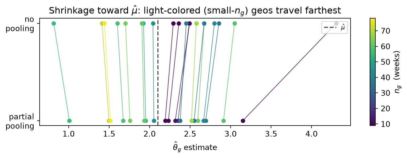
A1. Three-way pooling simulation with shrinkage plot. Simulate a scalar geo-MMM with G = 30 geographies. Draw week counts n_g independently and uniformly from \{4, 5, \ldots, 60\}; set \sigma^2 = 4.0 and \tau^2 = 1.0; draw true effects \theta_g \overset{\text{iid}}{\sim} \mathcal{N}(\mu, \tau^2) with \mu = 2.0; and generate group sample means \bar y_g \sim \mathcal{N}(\theta_g, \sigma^2/n_g). Implement three estimators. Complete pooling: estimate every \theta_g by the precision-weighted grand mean \hat\mu = (\sum_g (n_g/\sigma^2)\bar y_g)/(\sum_g n_g/\sigma^2). No pooling: estimate each \theta_g by \bar y_g. Empirical-Bayes partial pooling: set \hat\mu as above, estimate \hat\tau^2 = \max(0,\; \operatorname{Var}(\bar y_g) - n^{-1}\sum_g \sigma^2/n_g) (observed variance of the group means minus the average sampling variance, clamped at zero), then compute per-geography shrinkage weights \hat\lambda_g = (n_g/\sigma^2)/(n_g/\sigma^2 + 1/\hat\tau^2) and partial-pooled estimates \hat\theta_g^{\text{EB}} = \hat\lambda_g \bar y_g + (1 - \hat\lambda_g)\hat\mu. Compute total RMSE against the known \theta_g for all three methods and assert that partial pooling achieves strictly lower RMSE than both complete and no pooling. Produce a shrinkage plot: for each geography draw a line segment connecting its no-pooling estimate (at y = 1) to its partial-pooled estimate (at y = 0), colored by n_g; add a dashed vertical line at \hat\mu; verify visually that light-colored (small-n_g) geographies travel farther toward \hat\mu than dark (large-n_g) geographies. Then sweep \hat\tau^2 by replacing \tau^2_{\text{true}} with values \tau^2 \in \{0.01, 0.1, 0.5, 1.0, 4.0, 16.0\} in the data-generating process (holding \sigma^2, \mu, and the n_g fixed), refit partial pooling each time, and produce a second plot showing the partial-pooled estimates for the smallest-n_g geography as a function of \tau^2; describe how the shrinkage strength changes and explain the direction in terms of the shrinkage weight formula.
A2. Scalar hierarchical Gibbs sampler and closed-form verification. Simulate a scalar geo-MMM with G = 15 geographies: draw n_g uniformly from \{5, \ldots, 50\} (integer), set \sigma^2 = 4.0, \tau^2 = 1.0, \mu = 2.0, generate \theta_g \overset{\text{iid}}{\sim} \mathcal{N}(\mu, \tau^2) and \bar y_g \sim \mathcal{N}(\theta_g, \sigma^2/n_g). Implement a Gibbs sampler that cycles through the following conjugate full conditionals. (i) For each g = 1, \ldots, G in turn: given current (\mu, \tau^2, \sigma^2), draw \theta_g from \mathcal{N}(\hat m_g, v_g) where \hat m_g = \lambda_g \bar y_g + (1-\lambda_g)\mu, \lambda_g = (n_g/\sigma^2)/(n_g/\sigma^2 + 1/\tau^2), and v_g = \lambda_g \sigma^2/n_g. (ii) Given current \{\theta_g\} and \tau^2: draw \mu from \mathcal{N}(\bar\theta,\; \tau^2/G) with \bar\theta = G^{-1}\sum_g \theta_g. (iii) Given current \{\theta_g\} and \mu: draw \tau^2 from \mathcal{IG}(a_0 + G/2,\; b_0 + \tfrac{1}{2}\sum_g(\theta_g - \mu)^2) using weak hyperpriors a_0 = b_0 = 0.01. Run 25{,}000 Gibbs iterations and discard the first 5{,}000 as warm-up. Compute the Gibbs posterior mean of every \theta_g and compare it to the closed-form empirical-Bayes shrinkage estimate evaluated at the true hyperparameters (\mu = 2.0, \tau^2 = 1.0): assert that all G absolute deviations are below 0.15 and report the maximum deviation. Then explain in two sentences why the Gibbs posterior means do not match the closed-form shrinkage formula exactly, even with infinitely many samples: what additional source of uncertainty does the Gibbs sampler propagate that the closed-form empirical-Bayes estimate ignores, and why does that additional uncertainty make the full Bayesian approach more honest about the final coefficient estimates?