Motivation
Chapter 8 ends with a guarantee and a gap. Its ergodic theorem establishes that an irreducible, aperiodic Markov chain with stationary distribution \pi — one that is reversible with respect to \pi in the sense that the detailed-balance condition \pi(x)P(x,y) = \pi(y)P(y,x) holds for all state pairs — produces a trajectory whose time average \frac{1}{n}\sum_{t=1}^n f(X_t) converges almost surely to \mathbb{E}_\pi[f] regardless of the starting point, at a geometric rate set by the spectral gap 1 - |\lambda_2|. Its convergence theorem and the detailed-balance-implies-stationarity proof together identify exactly which structural property the chain must satisfy for the guarantee to hold. What Chapter 8 never does is build such a chain for a prescribed target. It analyzes chains — computes absorption probabilities, identifies the stationary distribution, bounds the mixing time — but the target \pi is always given by the problem and the kernel P is the object of analysis. This chapter inverts that stance entirely: the target \pi is the posterior distribution whose form you specify, and the kernel P is what you must construct. The question is how.
The urgency of that question is clearest at the boundary Chapter 5 identified. A Gaussian likelihood with a Gaussian prior over the regression coefficients \beta yields a posterior that is again Gaussian — p(\beta \mid y) \propto p(y \mid \beta)\,p(\beta) reduces to a standard normal integral and the posterior parameters are available in closed form.
That conjugacy breaks the moment the model acquires the features that make it a genuine MMM. Imposing a half-normal prior on media coefficients — enforcing that channel effects cannot be negative — changes the posterior’s support to a half-space and destroys conjugacy. Passing spend through an adstock transformation or a Hill saturation curve before multiplying by \beta introduces a nonlinearity that makes the likelihood non-Gaussian in \beta, and the posterior loses its named distributional form entirely.
In the hierarchical model of Chapter 6, the joint posterior p(\beta_{1:G}, \mu_\beta, \Sigma_\beta, \sigma^2 \mid y) is the product of conjugate-looking conditionals — each block’s full conditional remains tractable, which is why Gibbs sweeps work block by block — but the joint distribution itself is not any named distribution, and its normalizing constant, the marginal likelihood \int p(y \mid \beta)\,p(\beta)\,d\beta integrated over the full parameter space, is a high-dimensional integral with no closed form.
You can evaluate the unnormalized posterior p(y \mid \beta)\,p(\beta) at any particular \beta — that requires only a likelihood evaluation and a prior evaluation, both cheap — but you cannot integrate it, normalize it, or obtain exact draws from it by any elementary technique.
That asymmetry between evaluation and integration poses the chapter’s central question: the posterior is a formula you can evaluate at any \beta but cannot integrate, normalize, or sample from directly — so how do you draw from it? The answer is to manufacture a Markov chain whose stationary distribution is exactly that posterior, using nothing more than pointwise evaluations of the unnormalized density. The structural fact that makes this possible is the cancellation noted at the end of Chapter 8’s Rung 3: the detailed-balance condition \pi(x)P(x,y) = \pi(y)P(y,x) depends on the target only through the ratio \pi(y)/\pi(x), and any constant factor in \pi — including the intractable normalizing constant — divides out of that ratio identically.
The Metropolis–Hastings algorithm turns this observation into a general construction: given any proposal distribution q(x, y) from which you can draw candidate moves and evaluate densities, it defines an accept–reject rule for the proposal that enforces detailed balance with respect to \pi by design, producing a reversible kernel from any unnormalized target.
The Gibbs sampler of Chapter 6 is, as this chapter makes precise, a special case of the same principle: cycling through full conditionals p(\beta_g \mid \text{rest}) defines a transition that leaves the joint posterior invariant and satisfies detailed balance block by block, and its convergence — deferred in Chapter 6 with the promise that “the only missing ingredient is the theorem guaranteeing convergence” — is exactly the consequence of irreducibility, aperiodicity, and the ergodic theorem of Chapter 8, now paid in full.
Beyond the constructions themselves, the chapter develops the efficiency questions that govern practical sampler design: the acceptance rate, the autocorrelation between successive iterates, and the effective sample size, which converts a run of n correlated draws into the equivalent number of independent ones.
These quantities carry a pointed message for MMM: random-walk Metropolis–Hastings mixes slowly on the strongly correlated posteriors that collinear channel-spend data produces, because the correlation structure of the target concentrates probability along a narrow ridge that a symmetric random-walk proposal explores only at the cost of high autocorrelation and small effective sample size. Understanding precisely why this happens — and recognizing that it is a property of the geometry of \pi, not a defect of the Metropolis idea — is what motivates the Hamiltonian Monte Carlo of Chapter 10, which exploits the gradient of \log \pi to propose large, informed moves that traverse the posterior’s ridges efficiently.
Theory & Proofs
Two questions set the agenda for this chapter’s theory. First, why does Monte Carlo integration scale to high-dimensional posteriors while deterministic quadrature does not? Second, when the posterior cannot be sampled directly, how is a Markov chain engineered to sample it? Rung 1 answers the first and frames the second as the chapter’s central construction problem; Rung 2 delivers that construction in the Metropolis–Hastings algorithm and its keystone reversibility proof.
Rung 1 — The Monte Carlo principle and why MCMC
The Motivation closed with a precise question: given an unnormalized posterior that can be evaluated pointwise but not integrated, how do you draw samples from it? Before answering, it is worth understanding what those samples are for and why the task of drawing them is hard.
Monte Carlo estimation. Suppose, hypothetically, you could draw n independent samples X_1,\dots,X_n \sim \pi. The Monte Carlo estimator of \mathbb{E}_\pi[f] = \int f(x)\,\pi(x)\,\mathrm{d}x is the sample mean,
\hat\mu_n = \frac{1}{n}\sum_{i=1}^n f(X_i).
Linearity of expectation gives \mathbb{E}[\hat\mu_n] = \mathbb{E}_\pi[f] immediately — the estimator is unbiased for any \pi and any integrable f. Its variance is \operatorname{Var}(\hat\mu_n) = \sigma_f^2/n where \sigma_f^2 = \operatorname{Var}_\pi(f), so the standard deviation of the error is
\operatorname{std}(\hat\mu_n - \mathbb{E}_\pi[f]) = \frac{\sigma_f}{\sqrt{n}}.
By the central limit theorem, \sqrt{n}(\hat\mu_n - \mathbb{E}_\pi[f]) \xrightarrow{d} \mathcal{N}(0,\sigma_f^2), so the 1/\sqrt{n} rate is not merely a bound but an asymptotically sharp description of the estimator’s behavior.
Dimension freedom. The quantity \sigma_f/\sqrt{n} depends on the variance of f under \pi and on n, and on nothing else — in particular, not on the dimension p of the parameter space. This is the structural contrast with deterministic numerical quadrature. A tensor-product rule on a p-dimensional domain with m grid points per axis evaluates the integrand at m^p points and achieves an error of order m^{-r} for an integrand with r continuous derivatives; expressing the error in terms of the total number of evaluations n = m^p gives n^{-r/p}, a rate that degrades exponentially as p grows. Monte Carlo achieves n^{-1/2} regardless of p. For a posterior over G market-level regression vectors \beta_1,\dots,\beta_G each of dimension d, the full parameter space has dimension p = Gd — easily in the hundreds for a realistic hierarchical MMM — and the quadrature curse is immediately prohibitive. The 1/\sqrt{n} rate is the reason sampling is the tool of choice for high-dimensional Bayesian computation.
The obstacle: sampling from a complex posterior. The Monte Carlo argument presupposes i.i.d. draws from \pi. Obtaining such draws from an arbitrary posterior is a different matter. The simplest method — inverse-CDF sampling — requires the closed-form quantile function \pi^{-1}, which does not exist in more than one dimension. Rejection sampling draws from a proposal q that dominates \pi (i.e. \pi(x) \le M\,q(x) for all x) and accepts with probability \pi(x)/(M\,q(x)); the expected acceptance probability is 1/M, but finding a tight envelope requires knowing \pi globally, and in p dimensions the constant M necessarily grows exponentially in p as q and \pi diverge in their concentration — the curse of dimensionality applied to sampling. For the hierarchical MMM posterior, with its long ridge of correlated (\beta_g, \mu_\beta) values, rejection sampling is entirely impractical.
The resolution: dependent sampling via Markov chains. The key observation is that the Monte Carlo estimator \hat\mu_n is justified by independence of the draws, and that Chapter 8’s ergodic theorem removes the independence requirement entirely. Let X_1, X_2, \dots be an irreducible Markov chain with stationary distribution \pi. Then
\frac{1}{n}\sum_{t=1}^n f(X_t) \xrightarrow{\ \text{a.s.}\ } \mathbb{E}_\pi[f]
regardless of the dependence among the iterates, regardless of the starting point, and for any bounded f. The 1/\sqrt{n} Monte Carlo rate is replaced by a slightly slower rate that also involves the effective sample size n_{\mathrm{eff}} = n/(1 + 2\sum_{k \ge 1}\rho_k), which accounts for the autocorrelations \rho_k between draws k steps apart — a cost of dependence that later sections of this chapter quantify — but the essential conclusion stands: the law of large numbers holds for Markov-chain output. The entire problem therefore reduces to constructing a transition kernel P(x,\cdot) whose stationary distribution is exactly \pi. Chapter 8’s detailed-balance theorem identifies the key design tool: a kernel satisfying \pi(x)P(x,y) = \pi(y)P(y,x) for all state pairs has \pi as its stationary distribution, and the condition uses \pi only through the ratio \pi(y)/\pi(x), so the intractable normalizing constant cancels. Rung 2 delivers the construction.
Rung 2 — Metropolis–Hastings
The Metropolis–Hastings algorithm is a recipe for building a transition kernel P(x,\cdot) that satisfies detailed balance with respect to \pi by construction, using nothing more than pointwise evaluations of the unnormalized density \tilde\pi.
The algorithm. At step t, the chain is at state x = X_t. Draw a proposal y \sim q(\cdot \mid x), where q(y \mid x) is a probability density that the practitioner specifies freely. Compute the acceptance probability
\alpha(x,y) = \min\!\left(1,\ \frac{\pi(y)\,q(x\mid y)}{\pi(x)\,q(y\mid x)}\right),
then set
X_{t+1} = \begin{cases} y & \text{with probability } \alpha(x,y), \\ x & \text{with probability } 1 - \alpha(x,y). \end{cases}
For x \ne y, the off-diagonal transition density of the resulting kernel is
P(x,y) = q(y \mid x)\,\alpha(x,y),
and there is a complementary rejection mass at x itself — the diagonal term — equal to the total probability of rejection from state x: P(x,\{x\}) = 1 - \int P(x,y)\,\mathrm{d}y.
Theorem (Metropolis–Hastings is reversible). The Metropolis–Hastings kernel satisfies detailed balance with respect to \pi: \pi(x)P(x,y) = \pi(y)P(y,x) for all x \ne y. Hence, by Chapter 8’s detailed-balance theorem, \pi is a stationary distribution of the chain.
Proof. Fix x \ne y. Substitute P(x,y) = q(y\mid x)\,\alpha(x,y) and apply the elementary min identity: for any a, b > 0,
a\,\min(1,\,b/a) = \min(a,\,b).
Set a = \pi(x)\,q(y\mid x) and b = \pi(y)\,q(x\mid y). Then
\begin{aligned}
\pi(x)\,P(x,y)
&= \pi(x)\,q(y\mid x)\,\min\!\left(1,\frac{\pi(y)\,q(x\mid y)}{\pi(x)\,q(y\mid x)}\right) \\[6pt]
&= \min\!\bigl(\pi(x)\,q(y\mid x),\;\pi(y)\,q(x\mid y)\bigr).
\end{aligned}
The right-hand side is symmetric in x and y: swapping x \leftrightarrow y leaves \min(a,b) unchanged. Performing the identical computation starting from \pi(y)P(y,x),
\begin{aligned}
\pi(y)\,P(y,x)
&= \pi(y)\,q(x\mid y)\,\min\!\left(1,\frac{\pi(x)\,q(y\mid x)}{\pi(y)\,q(x\mid y)}\right) \\[6pt]
&= \min\!\bigl(\pi(y)\,q(x\mid y),\;\pi(x)\,q(y\mid x)\bigr),
\end{aligned}
which is the identical quantity. Therefore \pi(x)P(x,y) = \pi(y)P(y,x) for all x \ne y; the diagonal term satisfies detailed balance trivially (\pi(x)P(x,x) = \pi(x)P(x,x)). By Chapter 8’s detailed-balance-implies-stationarity theorem, \pi is stationary. \blacksquare
The normalizer cancels. The acceptance probability \alpha(x,y) involves \pi only through the ratio \pi(y)/\pi(x). If the target has the form \pi(x) = \tilde\pi(x)/Z for an intractable normalizing constant Z, then
\frac{\pi(y)}{\pi(x)} = \frac{\tilde\pi(y)/Z}{\tilde\pi(x)/Z} = \frac{\tilde\pi(y)}{\tilde\pi(x)},
and Z cancels identically. The Metropolis–Hastings algorithm therefore runs entirely on the unnormalized posterior \tilde\pi(\beta) = p(y \mid \beta)\,p(\beta) — the likelihood times the prior, both cheap to evaluate at any \beta — which is precisely the situation the Motivation identified: a formula evaluable pointwise but not integrable or normalizable.
Special cases. When the proposal is symmetric, q(y\mid x) = q(x\mid y), the proposal-density ratio cancels and the acceptance probability reduces to the original Metropolis rule:
\alpha(x,y) = \min\!\left(1,\ \frac{\pi(y)}{\pi(x)}\right).
The two standard instances are the random-walk Metropolis sampler, which sets y = x + \varepsilon with \varepsilon drawn from a symmetric density — e.g. \varepsilon \sim \mathcal{N}(0,s^2 I), so q(y\mid x) = q(x\mid y) because the density depends only on \|y - x\| — and the independence sampler, which proposes y \sim q(y) independently of the current state and applies the full Metropolis–Hastings ratio. Random-walk Metropolis is the default starting point in practice; its efficiency, measured by the acceptance rate and the resulting autocorrelation, depends critically on the step-size s relative to the posterior’s scale — a theme developed in detail when the effective sample size is introduced.
Convergence inherited from Chapter 8. The Metropolis–Hastings chain is a Markov chain, and Chapter 8’s convergence theorem and ergodic theorem apply whenever the chain is irreducible and aperiodic. A sufficient condition is that the proposal q(y\mid x) has positive density on the support of \pi for every x: any state y in the support of \pi can then be proposed from any x and accepted with positive probability \alpha(x,y) > 0, giving irreducibility; aperiodicity follows because the chain has positive probability of staying at x (rejection) at any step. Under these conditions the marginal distribution of X_t converges in total variation to \pi at a geometric rate set by the spectral gap, and the time-averages \frac{1}{n}\sum_{t=1}^n f(X_t) converge almost surely to \mathbb{E}_\pi[f] (Robert and Casella 2004).
The Metropolis–Hastings algorithm is the construction Chapter 8 promised but did not give. Given any posterior \pi(\beta) \propto p(y \mid \beta)\,p(\beta) that can be evaluated pointwise, it produces — through nothing more than a proposal draw, a ratio evaluation, and a Bernoulli accept–reject — a Markov chain whose stationary distribution is exactly \pi, whose convergence is guaranteed by Chapter 8’s theorems, and whose time-averages are consistent estimators of posterior expectations. This is the keystone that locks MCMC into place.
Rung 3 — The Gibbs sampler and its invariance proof
Metropolis–Hastings constructs a valid transition by appending an accept–reject filter to an arbitrary proposal. The Gibbs sampler takes a different path: it avoids the accept–reject step entirely by proposing from a distribution that is, by construction, exactly right for the local geometry of \pi. The price is that this perfectly calibrated proposal must be available in closed form. The payoff is that every proposal is accepted and no candidate move is ever wasted.
The algorithm. Partition the parameter vector into d blocks x = (x_1, \dots, x_d). One sweep replaces each block in turn: for i = 1, \dots, d, draw a fresh value x_i' from the full conditional
p(x_i \mid x_{-i}),
where x_{-i} = (x_1, \dots, x_{i-1}, x_{i+1}, \dots, x_d) denotes all blocks except block i, and hold all other blocks at their current values (x_{-i}' = x_{-i}). After all d updates in sequence the chain has completed one step, producing a new state (x_1', \dots, x_d'). This is systematic-scan Gibbs, with the blocks updated in a fixed order; an alternative is random-scan Gibbs, which at each step selects a block i uniformly at random and updates only that block, a device sometimes preferred for theoretical analysis. Both variants require the full conditionals in closed form — an algebraic tractability that is not always available, a point addressed at the end of this rung.
Theorem (Gibbs leaves \pi invariant). The full-conditional update of block i — draw x_i' \sim p(\cdot \mid x_{-i}), keep x_{-i}' = x_{-i} — preserves \pi: if the current state is distributed as \pi, so is the updated state.
Proof. The update changes only block i; the remaining blocks x_{-i} are untouched. The density of the updated state (x_i', x_{-i}) is obtained by averaging the old block x_i out of the joint and applying the conditional draw:
\begin{aligned}
\int \pi(x_i, x_{-i})\,p(x_i' \mid x_{-i})\,\mathrm{d}x_i
&= p(x_i' \mid x_{-i})\int \pi(x_i, x_{-i})\,\mathrm{d}x_i && \text{(factor out the draw)} \\
&= p(x_i' \mid x_{-i})\,\pi(x_{-i}) && \text{(marginalize $x_i$)} \\
&= \pi(x_i', x_{-i}) && \text{(conditional $\times$ marginal).}
\end{aligned}
The draw p(x_i' \mid x_{-i}) does not depend on the integration variable x_i, so it factors out; integrating \pi over block i leaves the marginal \pi(x_{-i}); and the product of conditional and marginal reconstitutes the joint. Thus the updated state has density \pi. \blacksquare
Gibbs is Metropolis–Hastings with acceptance probability 1. To see why, cast the full-conditional update as a Metropolis–Hastings step. The proposal is q(x' \mid x) = p(x_i' \mid x_{-i}) with x_{-i}' = x_{-i}, and the Metropolis–Hastings acceptance ratio is
\frac{\pi(x')\,q(x \mid x')}{\pi(x)\,q(x' \mid x)} = \frac{\pi(x_i', x_{-i})\,p(x_i \mid x_{-i})}{\pi(x_i, x_{-i})\,p(x_i' \mid x_{-i})}.
Substitute \pi(x_i', x_{-i}) = p(x_i' \mid x_{-i})\,\pi(x_{-i}) in the numerator and \pi(x_i, x_{-i}) = p(x_i \mid x_{-i})\,\pi(x_{-i}) in the denominator. Every factor cancels:
\frac{p(x_i' \mid x_{-i})\,\pi(x_{-i})\,p(x_i \mid x_{-i})}{p(x_i \mid x_{-i})\,\pi(x_{-i})\,p(x_i' \mid x_{-i})} = 1,
so \alpha \equiv 1: every Gibbs proposal is accepted. The Gibbs sampler is therefore the special case of Metropolis–Hastings whose proposals are never rejected precisely because they are drawn from the correct local conditional distribution.
Connection to Chapter 6. The hierarchical MMM sampler of Chapter 6 cycled through blocks \beta_g, \mu_\beta, \Sigma_\beta, and \sigma^2, drawing each from its conjugate full conditional while holding all other blocks fixed. That procedure is a Gibbs sampler. Chapter 6 deferred the formal justification for why the procedure works — why cycling conjugate draws eventually samples the joint posterior — with the promise that “the only missing ingredient is the theorem guaranteeing convergence.” The invariance proof above and Chapter 8’s ergodic theorem, applied to the Gibbs chain, are that missing ingredient, now paid in full.
When full conditionals are unavailable. Gibbs requires that each block’s full conditional be available in closed form. Conjugate priors and normal likelihoods supply this; nonconjugate priors or nonlinear likelihoods often do not. When a single block lacks a tractable full conditional, the pure Gibbs sweep can be augmented: replace that block’s Gibbs draw with a Metropolis–Hastings step targeting the full conditional of that block. The resulting hybrid is called Metropolis-within-Gibbs. The invariance argument extends immediately, since each block update — whether a direct Gibbs draw or a Metropolis step targeting the same full conditional — leaves \pi invariant, and the composition of invariance-preserving updates is again invariance-preserving.
Gibbs sampling is thus not a rival to Metropolis–Hastings but a highly efficient special case, available when the posterior’s block-conditional structure is exploitable. Both algorithms rest on the same detailed-balance guarantee, and both inherit convergence from Chapter 8’s ergodic theorem.
Rung 4 — Efficiency: acceptance, autocorrelation, and effective sample size
Rung 1 noted that the Monte Carlo estimator’s variance inflates when draws are correlated, replacing the i.i.d. standard error \sigma_f/\sqrt{n} with a larger quantity. This rung makes that inflation precise and connects it to the tuning decisions that govern practical sampler performance.
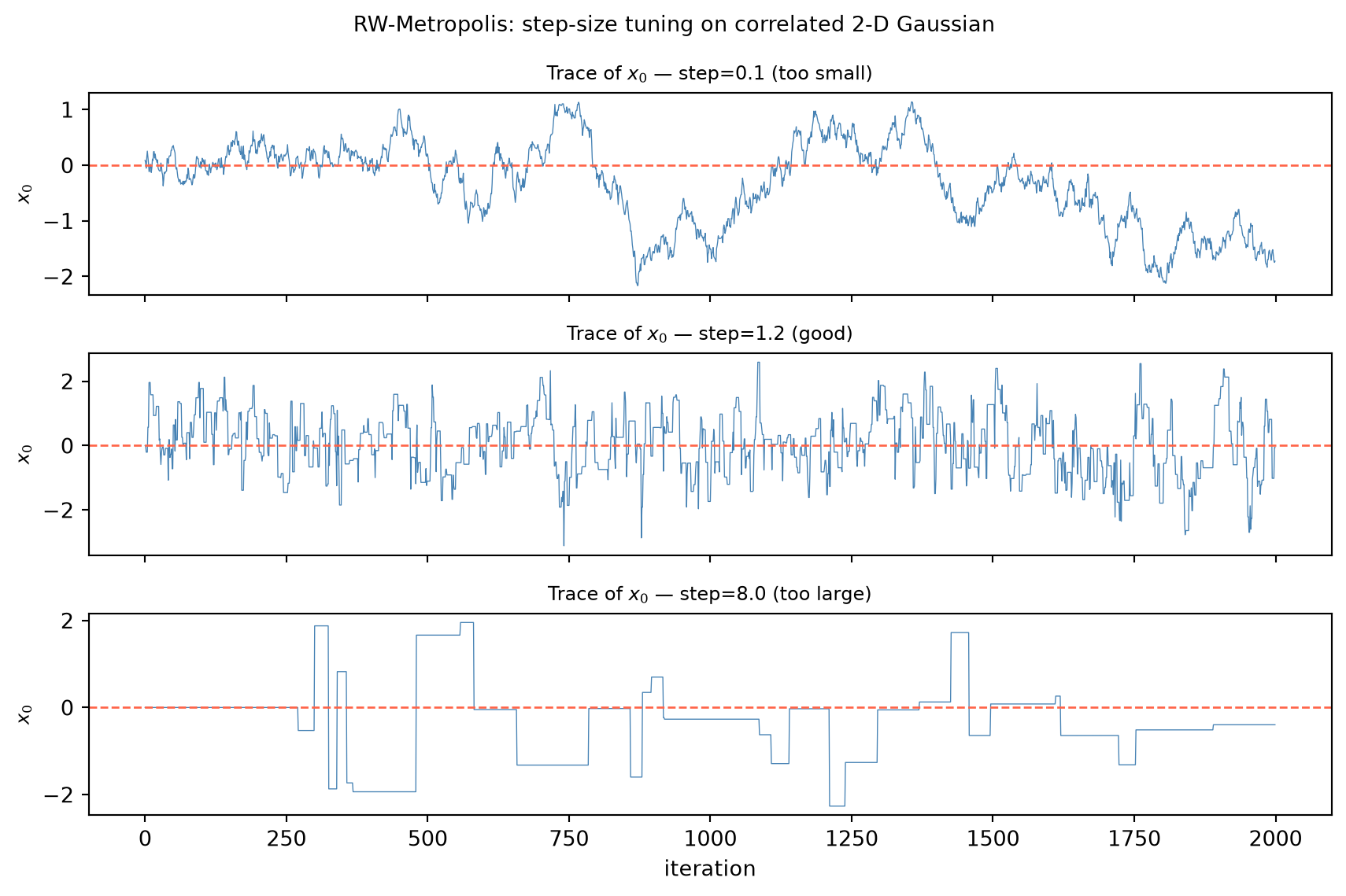
The step-size tradeoff for random-walk Metropolis. Dependent draws carry less information than independent ones — but how much less depends on how strong the dependence is, which in random-walk Metropolis is controlled almost entirely by the proposal step size s. When s is very small, nearly every proposal y = x + \varepsilon with \varepsilon \sim \mathcal{N}(0, s^2 I) lands close to the current state and inside the high-density region of \pi; the acceptance probability \alpha(x,y) is near 1, but each accepted move is tiny, so consecutive iterates are nearly identical and autocorrelation is high. When s is very large, proposals jump far from the current state and typically land in the low-density tails of \pi; most are rejected, and the chain stalls at one point for many consecutive steps, again producing high autocorrelation. Both extremes waste samples. An intermediate s — large enough to move meaningfully between iterations, small enough to keep the acceptance rate off the floor — achieves the best tradeoff. Quantifying that tradeoff requires measuring the autocorrelation the sampler induces.
Autocorrelation. Let f(X_t) be any scalar functional of the chain’s output, monitored across a run that has reached stationarity. The lag-k autocorrelation is
\rho_k = \operatorname{Corr}(f(X_t),\, f(X_{t+k})),
which, under stationarity, does not depend on t. For a random-walk Metropolis chain, the \rho_k are typically positive and decay geometrically in k at a rate set by the spectral gap; the slower the decay, the more the chain’s iterates resemble each other and the less independent information each one carries.
Effective sample size. The effective sample size (ESS) converts the information in n correlated draws into the equivalent number of independent draws:
\text{ESS} = \frac{n}{1 + 2\displaystyle\sum_{k \ge 1} \rho_k}.
The denominator \tau = 1 + 2\sum_{k \ge 1} \rho_k is the integrated autocorrelation time. The MCMC standard error of the time-average \hat\mu_n is
\operatorname{se}(\hat\mu_n) = \frac{\sigma_f}{\sqrt{\text{ESS}}},
which generalizes the i.i.d. formula \sigma_f/\sqrt{n}: when all \rho_k = 0 the chain is i.i.d. and \text{ESS} = n, recovering the classical rate. Positive autocorrelation, \rho_k > 0, inflates \tau above 1 and shrinks the effective sample size, so a chain of length n is worth only n/\tau independent draws. The ratio \tau can easily reach tens or hundreds in a poorly tuned sampler, meaning that ten thousand nominal posterior draws may carry the inferential content of only a few hundred independent ones.
Optimal acceptance rates. Optimal-scaling theory, which analyzes random-walk Metropolis in the limit of large dimension, identifies target acceptance rates that minimize integrated autocorrelation time. For a high-dimensional random-walk Metropolis targeting an isotropic posterior the optimal rate is approximately 0.234; in one dimension the corresponding target is approximately 0.44 (Robert and Casella 2004; Gelman et al. 2013). These heuristics are useful tuning targets: if the observed acceptance rate is well above 0.44, the step size is likely too small and the chain is making tiny, highly correlated moves; if it is well below 0.234, the step size is too large and the chain is stalling through repeated rejections. The argument that derives these numbers requires a functional central limit theorem for Markov chains and is not reproduced here; the practical upshot is a concrete dial — the proposal scale — that the practitioner can adjust while monitoring the acceptance rate.
Multi-chain diagnostics. The ESS defined here is a single-chain efficiency measure that quantifies how much the step-size choice is costing relative to an ideal i.i.d. sampler. Formal convergence diagnostics — the \hat R split-chain statistic and rank-normalized ESS, which diagnose whether multiple chains have converged to a common distribution — are the subject of Chapter 11. The code tie-in for this chapter optimizes step-size tuning using ESS as its efficiency criterion.
The effective sample size is the chapter’s core accounting unit: it converts the nominal length of a Markov-chain run into a quantity with the interpretive clarity of an independent sample size. Whether a posterior expectation is estimated reliably depends not on n but on \text{ESS}, and \text{ESS} depends on the autocorrelation structure that the sampler induces — which in turn depends on the sampler’s fit to the posterior’s geometry.
Rung 5 — Burn-in, mixing, and the bridge to Hamiltonian Monte Carlo
The ergodic theorem guarantees convergence of time-averages regardless of where the chain starts, but it is silent on how long the transient phase lasts. This rung examines that transient, explains why it is worst precisely on the posteriors that MMM produces, and identifies the structural remedy that motivates Chapter 10.
Burn-in and warm-up. A chain initialized at an arbitrary point X_0 is, in general, not yet distributed as \pi. By Chapter 8’s convergence theorem, the marginal distribution \mathcal{L}(X_t) approaches \pi geometrically at the spectral-gap rate: \|{\mathcal{L}(X_t) - \pi}\|_{\text{TV}} \le C(1-\gamma)^t where \gamma is the spectral gap. Until the chain has mixed, its iterates are biased toward the starting point and should not be used for posterior inference. The standard remedy is to discard the initial burn-in (or warm-up) period before computing any time-averages. The number of iterations to discard depends on the mixing time, which depends on the spectral gap, which depends on the geometry of \pi — the chain mixes in one step if \pi is a point mass and potentially never if the target is multimodal with deep valleys separating the modes.
Why random-walk Metropolis mixes slowly in high dimensions. In d dimensions, optimal-scaling theory establishes that to keep the acceptance rate from collapsing to zero as d \to \infty, the proposal standard deviation must scale like 1/\sqrt{d}. Proposals of size O(1/\sqrt{d}) move the chain by O(1/\sqrt{d}) per step; random-walking across a posterior of diameter O(1) therefore requires O(d) steps. A chain of fixed length n explores a shrinking fraction of the posterior as the parameter dimension grows.
The situation is substantially worse on strongly correlated posteriors. When probability concentrates along a narrow ridge — a cigar-shaped level set aligned with some direction in parameter space — an isotropic random-walk proposal that is agnostic to the ridge’s orientation faces a dilemma: proposals aligned with the ridge are small and barely move, while proposals perpendicular to the ridge are large and nearly always rejected. The result is a chain that drifts slowly along the ridge and rarely crosses it, producing high autocorrelation in the components that span the ridge and a small effective sample size. The upcoming Worked Example makes this concrete: in the bivariate-Gaussian Gibbs chain, the lag-1 autocorrelation of each coordinate equals \rho^2, the square of the target correlation between the two variables. As \rho \to 1 (near-degenerate posterior), \rho^2 \to 1, the autocorrelation time \tau diverges, and the effective sample size collapses to near zero for any fixed run length n.
The MMM connection. The MMM posterior exhibits exactly this pathology. Collinear channel-spend data — weeks in which several channels move together so that their individual effects cannot be distinguished from the data alone — produce a likelihood that constrains the sum of channel coefficients but not their individual values, generating a posterior ridge aligned with that sum. Chapter 4’s multicollinearity discussion described the problem in terms of inflated coefficient variance and high condition numbers; here the consequence is dynamical: the posterior concentrates along a ridge that an isotropic random walk explores at the cost of severe autocorrelation and a small effective sample size. More channels, more collinearity, more correlated posteriors — the curse compounds with model size.
The structural fix and the bridge to Chapter 10. The root cause of slow mixing is that a random-walk proposal is uninformed: it proposes moves symmetrically in all directions, without any knowledge of where \pi is large. The gradient \nabla \log \pi(x) carries exactly the missing information — it points in the direction of steepest ascent of the log-target and therefore toward the posterior’s high-density region. Hamiltonian Monte Carlo (HMC), the subject of Chapter 10, exploits that gradient by embedding the parameter vector in an augmented phase space with an auxiliary momentum variable and simulating Hamiltonian dynamics — a system that rolls the state along the posterior’s contours, making large, distant proposals that respect the ridge’s orientation and are accepted with high probability. Where random-walk Metropolis diffuses across the posterior in O(d) steps of size O(1/\sqrt{d}), HMC traverses it in O(d^{1/4}) steps of size O(1), a dramatic efficiency gain that becomes decisive on high-dimensional, correlated posteriors of exactly the kind that MMM produces. Chapter 11 then supplies the formal diagnostics — \hat R and rank-normalized ESS — that detect in practice whether a sampler, however sophisticated, has actually mixed.
The Theory section has now traced the full arc from the Monte Carlo principle, through the Metropolis–Hastings construction and its Gibbs specialization, to the efficiency measures that expose the cost of correlated draws, and finally to the geometric obstruction that makes gradient-informed proposals not a luxury but a necessity for realistic MMM inference.
Worked Examples
Example (a) — Metropolis acceptance by hand
The target is the unnormalized standard normal density,
\tilde\pi(x) = e^{-x^2/2},
with the normalizing constant 1/\sqrt{2\pi} deliberately dropped to show that the normalizer never enters any calculation. A symmetric random-walk proposal — draw y = x + \varepsilon from any density satisfying q(y\mid x) = q(x\mid y) — reduces the Metropolis–Hastings ratio to the original Metropolis rule (Rung 2):
\alpha(x,y) = \min\!\left(1,\ \frac{\tilde\pi(y)}{\tilde\pi(x)}\right) = \min\!\left(1,\ e^{-(y^2-x^2)/2}\right).
Three proposed moves are computed entirely by hand. In each case the exponent -(y^2 - x^2)/2 is all that is needed.
Move 1: x = 0 \to y = 1 (proposed move to lower density). The exponent is -(1^2 - 0^2)/2 = -0.5:
\alpha(0,\,1) = \min\!\left(1,\ e^{-0.5}\right) = e^{-0.5} \approx 0.6065.
The proposed point has lower density than the current state (\tilde\pi(1) = e^{-1/2} < \tilde\pi(0) = 1), so the ratio is below 1 and the move is accepted with probability 0.6065; otherwise the chain stays at 0.
Move 2: x = 1 \to y = 0.5 (proposed move to higher density). Now y^2 = 0.25 < x^2 = 1, so the exponent -(0.25 - 1)/2 = 0.375 is positive:
\alpha(1,\,0.5) = \min\!\left(1,\ e^{0.375}\right) = 1,
since e^{0.375} \approx 1.455 > 1. A move toward higher density is always accepted.
Move 3: x = 0.5 \to y = 2 (proposed far into the tail). The exponent is -(4 - 0.25)/2 = -1.875:
\alpha(0.5,\,2) = \min\!\left(1,\ e^{-1.875}\right) = e^{-1.875} \approx 0.1534.
The density at y = 2 is far smaller than at x = 0.5, and the chain accepts this distant tail move only about 15\% of the time.
Summary.
| 1 |
0 |
1 |
e^{-0.5} \approx 0.6065 |
0.6065 |
| 2 |
1 |
0.5 |
e^{0.375} \approx 1.455 |
1 (always accept) |
| 3 |
0.5 |
2 |
e^{-1.875} \approx 0.1534 |
0.1534 |
Interpretation. Three properties are visible at once. Uphill moves — proposals to states of higher unnormalized density — are always accepted; the chain freely explores toward the mode. Downhill moves are accepted in proportion to the density ratio, so the chain does visit the tails but spends less time there, weighting its visits in proportion to \tilde\pi. And crucially, the constant 1/\sqrt{2\pi} never appeared: it would have divided out of every ratio \tilde\pi(y)/\tilde\pi(x) identically, leaving nothing behind. By the detailed-balance proof of Rung 2, the long-run frequency with which the chain visits any region A converges to \int_A \pi(x)\,\mathrm{d}x — the properly normalized probability under \pi — without the normalizer ever being computed.
Example (b) — Gibbs sampling for the correlated bivariate normal
The target is the zero-mean bivariate normal \mathcal{N}(0, \Sigma) with
\Sigma = \begin{bmatrix} 1 & \rho \\ \rho & 1 \end{bmatrix}, \qquad \rho = 0.8,
so each variable has unit variance and the two share correlation 0.8 — the regime typical of nearly collinear channel-spend data in MMM. The Gibbs sampler alternates: draw x from its full conditional given the current y, then draw y from its full conditional given the new x.
Deriving the full conditionals. For \mathcal{N}(0,\Sigma) with unit marginal variances and correlation \rho, the standard Gaussian conditioning formula gives
\mathbb{E}[x \mid y] = \Sigma_{xy}\,\Sigma_{yy}^{-1}\,y = \frac{\rho}{1}\,y = \rho y,
\operatorname{Var}(x \mid y) = \Sigma_{xx} - \Sigma_{xy}\,\Sigma_{yy}^{-1}\,\Sigma_{yx} = 1 - \rho^2.
By symmetry the same formula holds for y \mid x, so the two full conditionals are
x \mid y \;\sim\; \mathcal{N}(\rho y,\ 1-\rho^2), \qquad y \mid x \;\sim\; \mathcal{N}(\rho x,\ 1-\rho^2).
With \rho = 0.8 the conditional variance is 1 - 0.64 = 0.36 and the conditional standard deviation is \sqrt{0.36} = 0.6. Every draw from a full conditional takes the form \rho \times (\text{conditioning value}) + 0.6\,Z for Z \sim \mathcal{N}(0,1).
Two Gibbs sweeps by hand. Start at (x_0, y_0) = (2, 2) — well away from the stationary mean of zero. To trace the deterministic skeleton of the chain, suppose each Z happens to equal 0, so each draw lands exactly at its conditional mean. (In a real sampler, each draw would add 0.6 \times Z for a genuinely random Z; the mean march below is the noiseless skeleton.)
Sweep 1.
Draw x_1 from \mathcal{N}(0.8 \times 2,\ 0.36) = \mathcal{N}(1.6,\ 0.36). With Z = 0: x_1 = 1.6.
Draw y_1 from \mathcal{N}(0.8 \times 1.6,\ 0.36) = \mathcal{N}(1.28,\ 0.36). With Z = 0: y_1 = 1.28.
Sweep 2.
Draw x_2 from \mathcal{N}(0.8 \times 1.28,\ 0.36) = \mathcal{N}(1.024,\ 0.36). With Z = 0: x_2 = 1.024.
Draw y_2 from \mathcal{N}(0.8 \times 1.024,\ 0.36) = \mathcal{N}(0.8192,\ 0.36). With Z = 0: y_2 = 0.8192.
Tracking the march toward the origin.
| 0 (start) |
2 |
2 |
| After sweep 1 |
1.6 |
1.28 |
| After sweep 2 |
1.024 |
0.8192 |
Each half-step multiplies the current mean by \rho = 0.8: the sequence of conditional means is 2 \to 1.6 \to 1.28 \to 1.024 \to 0.8192, a geometric series with ratio 0.8 converging to the stationary mean of 0. The higher the correlation \rho, the closer the ratio to 1 and the slower the march.
The mixing penalty. The lag-1 autocorrelation of either coordinate along the Gibbs chain equals \rho^2 = 0.64. Substituting into the integrated autocorrelation time, and using the geometric-series sum \sum_{k \ge 1} (\rho^2)^k = \rho^2/(1-\rho^2),
\tau = 1 + 2\sum_{k \ge 1} \rho^{2k} = 1 + \frac{2\rho^2}{1 - \rho^2} = 1 + \frac{2 \times 0.64}{0.36} \approx 4.56,
so n = 1{,}000 draws carry an effective sample size of only 1{,}000 / 4.56 \approx 219. As \rho \to 1, the lag-1 autocorrelation \rho^2 \to 1, the autocorrelation time \tau \to \infty, and the effective sample size collapses to near zero for any finite run length.
The MMM connection. Collinear channel-spend data (Chapter 4) produce posteriors where the coefficients of nearly co-moving channels are strongly correlated — the posterior concentrates along a ridge in coefficient space. A Gibbs sampler or random-walk Metropolis chain on such a posterior faces \rho close to 1, a lag-1 autocorrelation \rho^2 close to 1, and an autocorrelation time \tau large relative to any practical run length. The chain crawls along the ridge, generating a trace plot that drifts rather than mixes and a nominally large n that resolves to a disappointingly small ESS. Gradient-informed proposals — the subject of Chapter 10’s Hamiltonian Monte Carlo — exploit the direction of the posterior ridge directly, proposing along it rather than across it, and recover a practical ESS by sidestepping the geometry that defeats the simpler samplers.
Exercises
C – Conceptual / Reading Comprehension
C1. State the Monte Carlo principle: for i.i.d. draws X_i\sim\pi, the estimator \hat\mu_n=\frac1n\sum_i f(X_i) has standard error \sigma_f/\sqrt n. Explain why this rate is dimension-free and why that makes sampling preferable to deterministic quadrature for a high-dimensional MMM posterior (e.g. a hierarchical model with hundreds of coefficients). Then explain the obstacle — we cannot draw i.i.d. from a complex posterior — and why dependent draws from a Markov chain with stationary distribution \pi nonetheless yield a consistent estimator of \mathbb{E}_\pi[f]. Name the Chapter 8 theorem that licenses this.
C2. Write out the Metropolis–Hastings acceptance probability \alpha(x,y)=\min\!\big(1,\frac{\pi(y)q(x\mid y)}{\pi(x)q(y\mid x)}\big). Explain precisely why \pi enters only through the ratio \pi(y)/\pi(x), and why that means the unknown normalizing constant Z of a posterior \pi(\beta)=p(y\mid\beta)p(\beta)/Z never needs to be computed — the single property that makes MCMC applicable to the intractable posteriors of Chapter 5. Then state the condition on the proposal under which the ratio q(x\mid y)/q(y\mid x) drops out (the symmetric / Metropolis case), and give an example proposal for which it does not drop out.
C3. Explain why the Gibbs sampler is the special case of Metropolis–Hastings whose proposals — drawn from the full conditionals p(x_i\mid x_{-i}) — are accepted with probability 1, and how this identifies Chapter 6’s hierarchical sampler as a Gibbs sampler. Describe what Metropolis-within-Gibbs does when one block lacks a closed-form full conditional. Then explain what the acceptance rate, the autocorrelation \rho_k, and the effective sample size \text{ESS}=n/(1+2\sum_k\rho_k) each measure, and why random-walk Metropolis mixes slowly on the strongly correlated posteriors produced by collinear channel spends — the pathology that motivates Hamiltonian Monte Carlo.
B – By Hand
B1. For the unnormalized target \pi(x)\propto e^{-x^2/2} with a symmetric random-walk proposal, the Metropolis acceptance probability is \alpha(x,y)=\min(1,\,e^{-(y^2-x^2)/2}). Compute \alpha for each proposed move and state whether it is accepted with certainty or only probabilistically: (a) x=0\to y=1.5; (b) x=2\to y=1; (c) x=-1\to y=-2. (Answers: (a) e^{-1.125}\approx0.3247; (b) the move is to higher density, ratio >1, so \alpha=1; (c) e^{-1.5}\approx0.2231.)
B2. An asymmetric proposal, where the q-ratio does not cancel. The target is the unnormalized \pi(x)\propto e^{-x} on x>0 (an unnormalized \text{Exponential}(1)). The chain is at x=2 and proposes y=1, with proposal densities q(y\mid x)=q(1\mid 2)=0.5 and q(x\mid y)=q(2\mid 1)=0.2. Compute the full Hastings ratio and acceptance probability
\alpha(2,1)=\min\!\left(1,\ \frac{\pi(1)\,q(2\mid 1)}{\pi(2)\,q(1\mid 2)}\right)=\min\!\left(1,\ \frac{e^{-1}\cdot 0.2}{e^{-2}\cdot 0.5}\right),
and confirm \alpha=1 (the move is uphill in \pi, and the proposal correction only reinforces it). Then compute the acceptance probability of the reverse move — at x=1, propose y=2, with q(2\mid 1)=0.2 and q(1\mid 2)=0.5 —
\alpha(1,2)=\min\!\left(1,\ \frac{\pi(2)\,q(1\mid 2)}{\pi(1)\,q(2\mid 1)}\right)=\min\!\left(1,\ \frac{e^{-2}\cdot 0.5}{e^{-1}\cdot 0.2}\right),
report its value, and explain how the proposal asymmetry changes the answer relative to a symmetric proposal.
B3. A chain of n=10{,}000 draws has geometric autocorrelations \rho_k=0.6^k for k\ge1. Compute the integrated autocorrelation time
\tau=1+2\sum_{k\ge1}0.6^k=1+2\cdot\frac{0.6}{1-0.6},
and hence the effective sample size \text{ESS}=n/\tau. (Answer: \tau=1+2\cdot1.5=4, \text{ESS}=10{,}000/4=2{,}500.) Interpret: how many independent draws is this correlated chain worth, and by what factor is the MCMC standard error \sigma_f/\sqrt{\text{ESS}} larger than the i.i.d. \sigma_f/\sqrt n?
P – Prove It
P1. Prove that the Metropolis–Hastings kernel satisfies detailed balance with respect to \pi: for x\ne y with P(x,y)=q(y\mid x)\alpha(x,y) and \alpha(x,y)=\min\big(1,\frac{\pi(y)q(x\mid y)}{\pi(x)q(y\mid x)}\big), show \pi(x)P(x,y)=\pi(y)P(y,x). Use the identity a\min(1,b/a)=\min(a,b) with a=\pi(x)q(y\mid x), b=\pi(y)q(x\mid y), and the symmetry of \min(a,b) under x\leftrightarrow y. Conclude (citing Chapter 8) that \pi is stationary.
P2. Prove that a Gibbs full-conditional update leaves \pi invariant: for the update that draws x_i'\sim p(\cdot\mid x_{-i}) and keeps x_{-i} fixed, show that if the current state is distributed as \pi then so is the updated state, by marginalizing x_i out of the joint and re-applying the conditional (\int\pi(x_i,x_{-i})\,p(x_i'\mid x_{-i})\,dx_i=\pi(x_i',x_{-i})). Then prove Gibbs is Metropolis–Hastings with acceptance probability 1 by substituting the proposal q(x'\mid x)=p(x_i'\mid x_{-i}) into the Hastings ratio and showing it equals 1.
P3. (a) Derive the symmetric-proposal Metropolis special case \alpha(x,y)=\min(1,\pi(y)/\pi(x)) from the general Hastings ratio by imposing q(y\mid x)=q(x\mid y). (b) Derive the full conditional x\mid y\sim\mathcal N(\rho y,\,1-\rho^2) for the bivariate normal \mathcal N\!\big(0,\big[\begin{smallmatrix}1&\rho\\\rho&1\end{smallmatrix}\big]\big) — either by completing the square in x in the joint density, or by the Gaussian conditioning formula \mathbb E[x\mid y]=\Sigma_{xy}\Sigma_{yy}^{-1}y, \operatorname{Var}(x\mid y)=\Sigma_{xx}-\Sigma_{xy}\Sigma_{yy}^{-1}\Sigma_{yx}.
A – Applied / Code
A1. Tune a random-walk Metropolis sampler. Implement random-walk Metropolis for a target of your choice — e.g. the correlated 2-D Gaussian \mathcal N(0,[[1,0.8],[0.8,1]]), or a Bayesian linear-regression posterior. Sweep the proposal step size across a grid; for each, record the acceptance rate and an effective-sample-size estimate (from the summed autocorrelations of a monitored coordinate, truncated at the first negative lag). Plot acceptance rate and ESS versus step size, identify the efficient regime (acceptance roughly 0.2–0.5), and validate that the good-step sample mean and covariance match the known target. Comment on how the ESS-maximizing step relates to the heuristic optimal acceptance rate.
A2. Gibbs mixing and a non-conjugate posterior. (i) Implement Gibbs for the bivariate normal with the closed-form conditionals x\mid y\sim\mathcal N(\rho y,1-\rho^2); for \rho\in\{0.5,0.9,0.99\} measure the lag-1 autocorrelation and ESS of a coordinate, confirming the autocorrelation tracks \rho^2 and ESS collapses as \rho\to1. (ii) Sample a non-conjugate 1-D posterior with no closed form — e.g. a logistic / binary-conversion coefficient \beta with y_i\sim\text{Bernoulli}(\sigma(\beta x_i)) and prior \beta\sim\mathcal N(0,\tau^2), or a channel effect with a half-normal (non-negativity) prior — using random-walk Metropolis on the unnormalized log-posterior. Validate the MCMC histogram against a fine-grid normalized reference, confirming the sampler recovers a posterior Chapter 5 could not handle in closed form.