Theory & Proofs
The theory climbs a ladder, each rung resting on the one below. We begin with convex sets, the geometry of feasible regions; then convex functions, the shape of objectives; then the first- and second-order conditions that certify convexity without testing every pair of points. From these we prove the keystone — that every local minimum of a convex problem is global — and then carry it into the constrained setting through Lagrange multipliers and the KKT conditions, which deliver the budget capstone: the equal-marginal-returns rule for allocating spend. The section then ends at an honest reckoning with non-convexity, naming exactly what we lose when real response curves refuse to be concave. This part of the chapter builds the first two rungs — the sets and the functions — on which everything above is balanced.
Rung 1 — Convex sets
Every optimization problem searches over a region of allowable choices, and the geometry of that region decides whether the search is tractable. The simplest, most forgiving geometry is convexity: a set with no dents, no holes, and no disconnected pieces, so that you can never leave it by walking in a straight line from one member to another.
Definition. A set C \subseteq \mathbb{R}^n is convex if for all x, y \in C and every \lambda \in [0,1], the point \lambda x + (1-\lambda)y \in C. In words: the line segment between any two members of the set stays entirely inside the set. As \lambda sweeps from 0 to 1, the point \lambda x + (1-\lambda)y traces that segment from y to x, and convexity demands every point of it belong to C.
Examples that recur in optimization. Four convex sets appear again and again in what follows: a hyperplane \{x : a^\top x = b\}, a halfspace \{x : a^\top x \le b\}, a Euclidean norm ball \{x : \|x\| \le r\}, and a polyhedron \{x : Ax \le b\} — a finite intersection of halfspaces. The one we care about most is the budget feasible set
\mathcal{B} = \{\, b \in \mathbb{R}^n : b \ge 0,\ \mathbf{1}^\top b \le B \,\},
the set of nonnegative spend vectors whose total does not exceed the budget B. It is a polyhedron — in fact a simplex — and it is the region every budget optimizer in Part IV searches over.
Proposition (intersection preserves convexity). The intersection of any collection of convex sets is convex.
Proof. Let \{C_k\} be a collection of convex sets and take any x, y in the intersection \bigcap_k C_k, together with any \lambda \in [0,1]. For each index k, both x and y lie in C_k, and C_k is convex, so \lambda x + (1-\lambda)y \in C_k. Since this holds for every k, the point \lambda x + (1-\lambda)y lies in every C_k and hence in their intersection. The intersection therefore contains the segment between any two of its points, which is convexity. \blacksquare
Corollary. The budget feasible set \mathcal{B} is convex. It is the intersection of the n halfspaces \{b_i \ge 0\} — each one convex — and the single halfspace \{\mathbf{1}^\top b \le B\}, so the proposition applies directly. This is the feasible region every budget optimizer in Part IV searches over, and its convexity is precisely the hypothesis the later optimality theory will require.
Rung 2 — Convex functions
A convex feasible region is only half of what makes an optimization problem tractable; the other half is the shape of the objective being minimized over it. The right notion of shape is convexity of the function itself — a curvature condition that, married to a convex domain, is exactly what forces local searches to succeed.
Definition. A function f with convex domain is convex if for all x, y in the domain and every \lambda \in [0,1],
f(\lambda x + (1-\lambda)y) \le \lambda f(x) + (1-\lambda)f(y),
i.e. the chord joining (x, f(x)) and (y, f(y)) lies on or above the graph of f between them. The function is strictly convex if the inequality is strict whenever x \ne y and \lambda \in (0,1). The convex-domain requirement is not a technicality to be waved past: the left-hand side only makes sense if \lambda x + (1-\lambda)y is itself in the domain, so the inequality presupposes exactly the property Rung 1 established for \mathcal{B}.
Epigraph characterization. Convexity of a function reduces to convexity of a set. The epigraph of f is the region lying on or above its graph,
\text{epi}\,f = \{(x, t) : f(x) \le t\},
and f is convex if and only if \text{epi}\,f is a convex set (Boyd and Vandenberghe 2004). The equivalence is geometric: the chord-above-the-graph inequality says exactly that the segment joining two points of the epigraph stays inside the epigraph, which is the definition of a convex set. This is the bridge that lets every theorem about convex sets be read as a theorem about convex functions, and conversely.
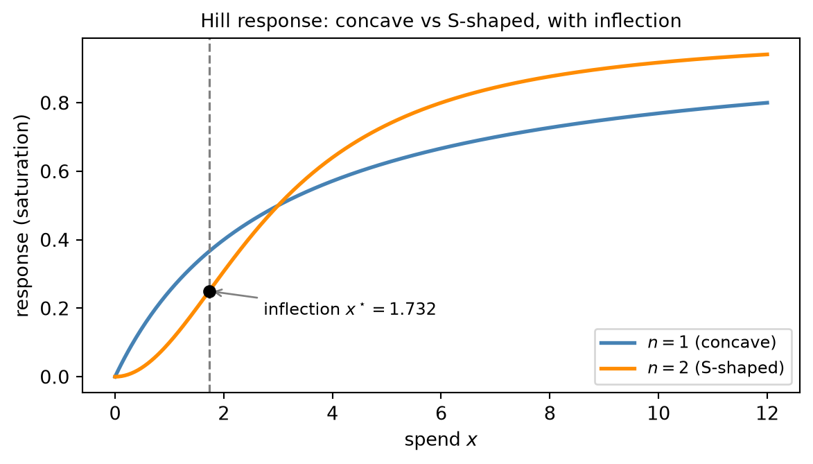
Concavity and the reduction to one theory. A function f is concave if -f is convex; equivalently, the chord lies on or below the graph. A diminishing-returns response curve is concave: each additional dollar of spend buys a little less than the last, so the graph bends downward. The canonical example is the Hill saturation curve introduced in Chapter 15,
f(x; K, n) = \frac{x^n}{K^n + x^n},
which for exponent n = 1 is concave in spend x \ge 0 — the textbook shape of an advertising channel that saturates. Concavity and convexity are not two theories but one, and the bridge is a single observation: maximizing a concave function is identical to minimizing its convex negative, since \arg\max_x f(x) = \arg\min_x \bigl(-f(x)\bigr) and the optimal value merely changes sign. So the budget problem’s “concave maximization” and the standard “convex minimization” are the same problem wearing different clothes. We therefore state every result for the convex-minimization side, without loss of generality, and read it off for concave maximization whenever the MMM demands it.
Rung 3 — The first-order condition
The chord definition of Rung 2 is exact but operationally hopeless: to certify a function convex by it, you would have to check the inequality for every pair of points and every \lambda between them — an infinite verification with no obvious starting place. When f is differentiable, there is a far cheaper test, one that examines the function a single point at a time through its gradient. It replaces a global statement about chords with a local statement about tangents.
Theorem (first-order condition). Let f be differentiable on a convex domain. Then f is convex if and only if
f(y) \ge f(x) + \nabla f(x)^\top (y - x) \quad \text{for all } x, y \text{ in the domain.}
Geometrically, the graph of f lies on or above each of its tangent planes: no matter where you take the tangent, the whole surface stays above it.
Proof. We argue both directions.
(\Rightarrow) Assume f is convex. Fix x, y in the domain and take \lambda \in (0,1]. Writing x + \lambda(y - x) = \lambda y + (1-\lambda)x, convexity gives
f\bigl(x + \lambda(y - x)\bigr) \le (1-\lambda)f(x) + \lambda f(y).
Subtract f(x) from both sides and divide by \lambda > 0:
\frac{f\bigl(x + \lambda(y - x)\bigr) - f(x)}{\lambda} \le f(y) - f(x).
As \lambda \to 0^+ the left-hand side converges to the directional derivative of f at x in the direction y - x, which is \nabla f(x)^\top (y - x). Taking the limit preserves the inequality, so \nabla f(x)^\top (y - x) \le f(y) - f(x), and rearranging gives the claimed tangent inequality.
(\Leftarrow) Assume the tangent inequality holds for every pair of points. Fix x, y and \lambda \in [0,1], and set z = \lambda x + (1-\lambda)y, which lies in the domain by convexity. Apply the inequality at the base point z to each endpoint:
\begin{aligned}
f(x) &\ge f(z) + \nabla f(z)^\top (x - z), \\
f(y) &\ge f(z) + \nabla f(z)^\top (y - z).
\end{aligned}
Form the combination \lambda \cdot (\text{first}) + (1-\lambda) \cdot (\text{second}). The gradient terms collect into \nabla f(z)^\top\bigl(\lambda x + (1-\lambda)y - z\bigr) = \nabla f(z)^\top (z - z) = 0, and the constant terms sum to f(z). What remains is
\lambda f(x) + (1-\lambda) f(y) \ge f(z) = f\bigl(\lambda x + (1-\lambda)y\bigr),
which is exactly the chord inequality defining convexity. \blacksquare
This condition is more than a verification tool; it carries the seed of the whole optimization story. At a stationary point, where \nabla f(x) = 0, the tangent term vanishes and the inequality collapses to f(y) \ge f(x) for every y in the domain — the stationary point is a global minimum. That single line is the keystone Rung 7 will state and prove in full.
Rung 4 — The second-order condition
The first-order condition tests convexity through the gradient, but for a twice-differentiable function there is an even more intrinsic test, one that speaks the native language of shape: curvature. A convex function curves upward everywhere, and curvature is precisely what the second derivative measures. In several variables the second derivative is the Hessian matrix \nabla^2 f, and the condition becomes a statement about its eigenvalues.
Theorem (second-order condition). Let f be twice continuously differentiable on an open convex domain. Then f is convex if and only if its Hessian is positive semidefinite everywhere: \nabla^2 f(x) \succeq 0 for all x in the domain. If \nabla^2 f(x) \succ 0 everywhere, then f is strictly convex.
Proof. The argument reduces the multivariate claim to a one-dimensional fact by slicing along lines.
A function on a convex domain is convex if and only if its restriction to every line is convex — the chord inequality only ever involves the two points x, y and the segment between them, all of which lie on a single line. So fix a base point x and a direction v, and define the scalar function g(t) = f(x + tv) on the interval of t for which x + tv stays in the domain. Differentiating through the chain rule twice gives
\begin{aligned}
g'(t) &= \nabla f(x + tv)^\top v, \\
g''(t) &= v^\top \nabla^2 f(x + tv)\, v.
\end{aligned}
Now invoke the one-dimensional fact: a twice-differentiable g is convex if and only if g''(t) \ge 0 everywhere. This follows from the first-order condition applied to g — convexity is equivalent to g' being nondecreasing, and by the mean value theorem g' is nondecreasing exactly when g'' \ge 0.
Stitching the slices back together, f is convex iff g is convex for every choice of x and v, iff g''(t) = v^\top \nabla^2 f(x + tv)\, v \ge 0 for all x, v, t, iff v^\top \nabla^2 f(x)\, v \ge 0 for all x and all v. That last statement is precisely the definition of the Hessian being positive semidefinite, \nabla^2 f(x) \succeq 0, reusing the PSD characterization from Chapter 1. If the inequalities are strict for v \ne 0, each slice is strictly convex and so is f. \blacksquare
Application to the Hill curve. The second-order condition turns the abstract question “is the response curve concave?” into a concrete derivative computation. Take the Hill curve f(x; K, n) = x^n / (K^n + x^n) and read its curvature off the sign of f''(x) for x > 0.
For n = 1 the curve simplifies to f(x) = x/(K + x), and a direct computation gives
f''(x) = -\frac{2K}{(K + x)^3} < 0 \quad \text{for all } x > 0.
The second derivative is strictly negative throughout, so f is strictly concave — the clean diminishing-returns shape in which every dollar buys less than the last, and the budget problem stays convex.
For n > 1 the story changes. The second derivative is a messier rational function, but the load-bearing fact is its sign: f'' is positive near the origin and negative far out, so it changes sign exactly once. The crossing — the inflection point where f''(x) = 0 — sits at
x^\star = K\left(\frac{n-1}{n+1}\right)^{1/n},
so f is convex on the “toe” 0 \le x < x^\star and concave for x > x^\star. For n = 2,\ K = 3 this gives x^\star = \sqrt{3} \approx 1.7321. This S-shape — convex toe, concave tail — is the seed of the trouble that Rung 10 confronts head-on: a response curve that is not globally concave makes the budget-allocation problem not globally convex, and a single descent can stall in the wrong basin.
Rung 5 — Operations that preserve convexity
Certifying a single function convex — by the chord definition, the tangent inequality, or the Hessian — is a self-contained exercise. But real objectives are never handed to us as one tidy function. They are built up from pieces: a sum of per-channel costs, a data-fit term plus a regularizer, a worst-case taken over scenarios. Re-deriving convexity from scratch for each composite would be wasteful when the pieces are already known to be convex. What we want instead is a small calculus of convexity — a handful of operations that, applied to convex inputs, are guaranteed to return convex outputs. With it, we certify the whole from the parts and never touch a Hessian for the assembled objective at all.
The toolkit. Four operations carry almost all the weight in practice:
- (i) Nonnegative weighted sums. If f_1, \dots, f_m are convex and w_1, \dots, w_m \ge 0, then \sum_i w_i f_i is convex.
- (ii) Composition with an affine map. If f is convex and g(x) = f(Ax + b), then g is convex.
- (iii) Pointwise maximum / supremum. If f_1, \dots, f_m are convex, then \max_i f_i is convex; more generally the pointwise supremum \sup_{\alpha} f_\alpha of any family of convex functions is convex.
- (iv) Scalar composition. If h is convex and nondecreasing and g is convex, then the composition h \circ g is convex.
We prove the first two — the rules that the book’s objectives lean on directly — and cite the standard reference for the rest.
Proof of (i) and (ii). Take any x, y in the relevant domain and any \lambda \in [0,1].
(i) Nonnegative weighted sums. Each f_i is convex, so its chord inequality holds:
f_i\bigl(\lambda x + (1-\lambda)y\bigr) \le \lambda f_i(x) + (1-\lambda)f_i(y).
Multiply both sides by w_i \ge 0 — a nonnegative factor preserves the direction of the inequality — and sum over i = 1, \dots, m:
\sum_i w_i f_i\bigl(\lambda x + (1-\lambda)y\bigr) \le \lambda \sum_i w_i f_i(x) + (1-\lambda)\sum_i w_i f_i(y).
Writing F = \sum_i w_i f_i, this reads F\bigl(\lambda x + (1-\lambda)y\bigr) \le \lambda F(x) + (1-\lambda)F(y), which is exactly the chord inequality for F. Hence \sum_i w_i f_i is convex.
(ii) Composition with an affine map. Let g(x) = f(Ax + b) with f convex, and set u = Ax + b, v = Ay + b. Because the map x \mapsto Ax + b is affine, it commutes with convex combinations:
A\bigl(\lambda x + (1-\lambda)y\bigr) + b = \lambda(Ax + b) + (1-\lambda)(Ay + b) = \lambda u + (1-\lambda)v.
Therefore, using convexity of f on the points u, v,
g\bigl(\lambda x + (1-\lambda)y\bigr) = f\bigl(\lambda u + (1-\lambda)v\bigr) \le \lambda f(u) + (1-\lambda)f(v) = \lambda g(x) + (1-\lambda)g(y),
which is the chord inequality for g. Hence g is convex. \blacksquare
Rules (iii) and (iv), stated. The remaining two follow the same spirit and we record them as facts (Boyd and Vandenberghe 2004). For the pointwise supremum (iii), the epigraph of \sup_\alpha f_\alpha is the intersection \bigcap_\alpha \text{epi}\,f_\alpha of the individual epigraphs; each is convex by the epigraph characterization of Rung 2, and intersections of convex sets are convex by Rung 1, so the supremum is convex. For scalar composition (iv), monotonicity is what makes it work: since h is nondecreasing, the chord inequality for g may be pushed through h without reversing, and then the convexity of h finishes the bound — so h \circ g is convex.
Payoff: ridge / MAP estimation is convex. The toolkit lets us certify a built-up objective without computing a single second derivative of the whole. Recall the negative log-posterior of Chapter 5’s Gaussian (ridge) model,
J(\beta) = \frac{1}{2\sigma^2}\|y - X\beta\|^2 + \frac{1}{2\tau^2}\|\beta\|^2,
whose minimizer is the MAP estimate. Read it through the calculus. The squared Euclidean norm \|\cdot\|^2 is convex (its Hessian is 2I \succ 0). The first term is that convex function composed with the affine map \beta \mapsto y - X\beta, hence convex by (ii); the second is \|\cdot\|^2 composed with the affine — indeed linear — identity map, hence convex by (ii) again. Finally J is the nonnegative weighted sum of these two convex pieces, with weights 1/(2\sigma^2) \ge 0 and 1/(2\tau^2) \ge 0, so it is convex by (i). Therefore MAP / ridge estimation is a convex optimization problem. The keystone of Rung 7 will then guarantee that its unique minimizer is global — and that minimizer is precisely the closed-form ridge solution \hat\beta = (X^\top X + \tfrac{\sigma^2}{\tau^2} I)^{-1} X^\top y derived by pure linear algebra in Part II. Part IV’s curvature theory and Part II’s algebra are describing the same point from two directions.
Rung 6 — Jensen’s inequality
The chord inequality of Rung 2 compares a convex function evaluated at a two-point average, \lambda x + (1-\lambda)y, to the corresponding average of its values. But an average over two points with weights \lambda and 1-\lambda is just the simplest probability distribution — a coin flip. Nothing in the geometry of convexity is special to two points, and the natural generalization replaces the finite average by an expectation over any probability distribution. That generalization is Jensen’s inequality, and it is the bridge from convexity to probability that the rest of the book will cross repeatedly.
Theorem (Jensen’s inequality). Let f be convex and let X be a random vector with finite mean \mu = \mathbb{E}[X], taking values in the domain of f. Then
f(\mathbb{E}[X]) \le \mathbb{E}[f(X)].
For concave f the inequality reverses.
Proof. Assume f is differentiable and apply the first-order condition of Rung 3 with base point \mu. For every realization x that X may take, the graph lies above the tangent plane at \mu:
f(X) \ge f(\mu) + \nabla f(\mu)^\top (X - \mu),
an inequality that holds pointwise, for each outcome of the random vector. Now take expectations of both sides. Expectation is monotone (it preserves \ge) and linear, and f(\mu) and \nabla f(\mu) are constants, so
\begin{aligned}
\mathbb{E}[f(X)] &\ge f(\mu) + \nabla f(\mu)^\top \mathbb{E}[X - \mu] && \text{(take expectations)} \\
&= f(\mu) && (\mathbb{E}[X - \mu] = 0) \\
&= f(\mathbb{E}[X]), && (\mu = \mathbb{E}[X])
\end{aligned}
which is the claim. If f is convex but not differentiable, the identical argument runs with a subgradient at \mu in place of \nabla f(\mu), since the supporting-hyperplane inequality holds there too. The concave case follows by applying the result to -f. \blacksquare
MMM reading: volatility is a tax. The response curve r is concave, so Jensen runs the other way:
r(\mathbb{E}[\text{spend}]) \ge \mathbb{E}[r(\text{spend})].
Read the two sides as two flighting plans with the same average budget. The left side is steady spend held at the average level; the right side is erratic spend — feast one week, famine the next — that merely averages out to the same total. Jensen says the steady plan produces at least as much expected response as the volatile one. Concavity penalizes volatility, and the size of the gap between the two sides is a quantitative measure of that penalty: it grows with the curvature of r, that is, with the strength of diminishing returns. This is the formal reason a smooth, level flighting plan beats a feast-or-famine one at equal total budget — and why, when Chapter 14 allocates spend, it is solving for the level plan rather than chasing spikes.
Rung 7 — The keystone: every local minimum is global
Rungs 1–6 built the machinery: convex sets, the chord and tangent characterizations of convex functions, the Hessian test, the closure rules, and Jensen. This rung is what all of it was for. A single structural property of convex functions is the reason convex optimization is tractable at all — and it is the reason detecting convexity, through the first- and second-order conditions of Rungs 3–4, is the opening move on any optimization problem. The foreshadowing planted at the end of Rung 3 is paid off here in full.
Theorem (local = global). Let f be convex on a convex set C. Then:
- every local minimizer of f over C is a global minimizer;
- if f is differentiable, the stationarity condition \nabla f(x^\star)^\top (y - x^\star) \ge 0 for all y \in C — which for an interior or unconstrained minimum reduces to \nabla f(x^\star) = 0 — is sufficient for x^\star to be a global minimizer;
- if f is strictly convex, the global minimizer is unique.
Proof.
Part 1 (local \Rightarrow global), by contradiction. Suppose x^\star is a local minimizer but not global, so there exists z \in C with f(z) < f(x^\star). For \lambda \in (0,1] consider the point x_\lambda = \lambda z + (1-\lambda)x^\star, which lies in C by convexity of the set. By convexity of f,
\begin{aligned}
f(x_\lambda) &\le \lambda f(z) + (1-\lambda)f(x^\star) && \text{(convexity of $f$)} \\
&= f(x^\star) + \lambda\bigl(f(z) - f(x^\star)\bigr) && \text{(rearrange)} \\
&< f(x^\star), && (f(z) < f(x^\star))
\end{aligned}
As \lambda \to 0^+, x_\lambda \to x^\star, so every neighborhood of x^\star contains points x_\lambda with f(x_\lambda) < f(x^\star) — contradicting that x^\star is a local minimizer. Hence no such z exists and x^\star is global.
Part 2 (stationarity is sufficient). Suppose \nabla f(x^\star)^\top(y - x^\star) \ge 0 for all y \in C. By the first-order condition of Rung 3, for every y \in C,
f(y) \ge f(x^\star) + \nabla f(x^\star)^\top(y - x^\star) \ge f(x^\star),
so x^\star is a global minimizer. For an unconstrained problem — or an interior minimizer, where y may be perturbed from x^\star in every direction — the condition \nabla f(x^\star)^\top(y - x^\star) \ge 0 for all directions forces \nabla f(x^\star) = 0, since a nonzero gradient would make the inner product negative along its own negative.
Part 3 (strict convexity \Rightarrow uniqueness). Suppose x^\star \ne x^{\star\star} are both global minimizers, so f(x^\star) = f(x^{\star\star}) = p^\star. The midpoint m = \tfrac12 x^\star + \tfrac12 x^{\star\star} lies in C by convexity, and strict convexity gives
f(m) < \tfrac12 f(x^\star) + \tfrac12 f(x^{\star\star}) = p^\star,
contradicting that p^\star is the minimum value of f over C. Hence the minimizer is unique. \blacksquare
Significance. This is why convex optimization works. A descent method that stops where it can no longer go downhill has, for a convex problem, found the global optimum — not a local trap. There is no need to restart from many initial points, no anxiety about whether the algorithm settled in the best basin: local information at a single stationary point certifies a global fact about the whole domain. Part 2 makes this operational, turning the search for a global optimum into the algebraic problem of solving \nabla f(x^\star) = 0, and Part 3 tells us exactly when the answer is the only one.
This also explains the workflow of all of Part IV. The first question to ask about any optimization problem is not “what algorithm should I run?” but “is this problem convex?”, because a yes converts local search into a global guarantee — it changes what a stopping point means. The first- and second-order conditions of Rungs 3–4 are precisely how that question gets answered, which is why we spent so long sharpening them.
And a forewarning. The guarantee is a property of convexity, not a law of nature. When the response curve is S-shaped — convex toe, concave tail, the very shape glimpsed in Rung 4 and confronted head-on in Rung 10 — the objective is no longer convex, and this keystone evaporates. A single descent can then halt in a local basin that is nowhere near the best, with no way to tell from local information alone that anything is wrong. That single failure is what forces the multi-start machinery of Chapter 14: when local can no longer certify global, the only recourse is to search many basins and compare.
Rung 8 — Constrained optimality: Lagrange and KKT
The keystone of Rung 7 is a theorem about unconstrained minimization: set the gradient to zero and, for a convex objective, you have the global optimum. But the budget problem is not unconstrained. Spend is nonnegative, and it must sum to (or stay within) the budget. Constraints change what “optimal” means. At a constrained optimum the gradient of the objective need not vanish — pushing further downhill may simply be forbidden by a constraint. What must instead hold is a balance: the objective’s gradient must be exactly cancelled by a combination of the constraint gradients, so that no feasible direction descends. Lagrange multipliers and the Karush–Kuhn–Tucker (KKT) conditions are the apparatus that formalizes that balance, and they are the bridge from Rung 7 to every constrained optimizer in Part IV.
The setup. Write the convex program in standard form,
\min_x\ f(x) \quad \text{subject to} \quad g_i(x) \le 0\ (i = 1, \dots, m), \quad h_j(x) = 0\ (j = 1, \dots, p),
with f and every g_i convex and every h_j affine. These hypotheses are exactly what make the program convex: the inequality sets \{g_i \le 0\} are convex sublevel sets of convex functions, the equality sets \{h_j = 0\} are hyperplanes, and the feasible region is their intersection — convex by Rung 1.
The device that couples objective and constraints is the Lagrangian, which attaches a scalar multiplier to each constraint and folds the whole problem into a single function:
L(x, \lambda, \nu) = f(x) + \sum_{i=1}^m \lambda_i g_i(x) + \sum_{j=1}^p \nu_j h_j(x), \qquad \lambda_i \ge 0,\ \nu_j \in \mathbb{R}.
The sign convention is not arbitrary. An inequality multiplier \lambda_i is constrained to be nonnegative: it prices a one-sided constraint g_i \le 0, and charging a penalty \lambda_i g_i that only bites when the constraint is pushed toward violation (g_i \to 0^+) requires \lambda_i \ge 0, so that relaxing the constraint can never look worse than respecting it. An equality multiplier \nu_j is free in sign, because an equality constraint can be violated in either direction and the penalty \nu_j h_j must be able to push back both ways.
The KKT conditions. A point (x^\star, \lambda^\star, \nu^\star) satisfies the KKT conditions when all four of the following hold:
- Stationarity: \nabla f(x^\star) + \sum_i \lambda_i^\star \nabla g_i(x^\star) + \sum_j \nu_j^\star \nabla h_j(x^\star) = 0. The objective gradient is balanced by a weighted sum of constraint gradients — no net pull remains.
- Primal feasibility: g_i(x^\star) \le 0 for all i and h_j(x^\star) = 0 for all j. The candidate point actually obeys the constraints.
- Dual feasibility: \lambda_i^\star \ge 0 for all i. The inequality prices respect the sign convention.
- Complementary slackness: \lambda_i^\star\, g_i(x^\star) = 0 for every i.
Complementary slackness deserves a word, because it is the condition that encodes which constraints matter. For each i the product \lambda_i^\star g_i(x^\star) is zero, so at least one factor must vanish. Either the constraint is active — it holds with equality, g_i(x^\star) = 0, and its multiplier \lambda_i^\star is free to be positive, exerting force on the optimum — or it is inactive, g_i(x^\star) < 0, with strict slack, and then complementary slackness forces \lambda_i^\star = 0. An inactive constraint exerts no force: it is not touching the optimum, so it contributes nothing to the stationarity balance. The multipliers thus switch off automatically for the constraints that do not bind.
Theorem (KKT sufficiency for convex programs). For the convex program above — f and all g_i convex, all h_j affine — if (x^\star, \lambda^\star, \nu^\star) satisfies the four KKT conditions, then x^\star is a global minimizer of f over the feasible set.
Proof. Fix the multipliers at their KKT values and define the partial Lagrangian
\tilde L(x) = f(x) + \sum_i \lambda_i^\star g_i(x) + \sum_j \nu_j^\star h_j(x),
a function of x alone. The proof has two moves: show \tilde L is globally minimized at x^\star by reducing to the keystone, then convert that into a statement about f on the feasible set.
Step 1: \tilde L is convex. The first term f is convex by hypothesis. Each term \lambda_i^\star g_i is a nonnegative multiple — \lambda_i^\star \ge 0 by dual feasibility — of a convex g_i, hence convex. Each term \nu_j^\star h_j is a scalar multiple of an affine function, hence affine and so convex. By the nonnegative-weighted-sum and affine rules of Rung 5, \tilde L is a sum of convex pieces and is therefore convex on \mathbb{R}^n.
Step 2: x^\star globally minimizes \tilde L. Differentiating \tilde L gives exactly the left-hand side of the stationarity condition, so KKT stationarity says \nabla \tilde L(x^\star) = 0. A convex function with a zero gradient is at a global minimum — this is precisely the keystone of Rung 7, Part 2, applied to the unconstrained convex function \tilde L. Hence
\tilde L(x) \ge \tilde L(x^\star) \quad \text{for all } x \in \mathbb{R}^n.
Step 3: transfer to f on the feasible set. Let y be any feasible point, so g_i(y) \le 0 and h_j(y) = 0. Then
\begin{aligned}
f(y) &\ge f(y) + \sum_i \lambda_i^\star g_i(y) + \sum_j \nu_j^\star h_j(y) = \tilde L(y) \\
&\ge \tilde L(x^\star) = f(x^\star) + \sum_i \lambda_i^\star g_i(x^\star) + \sum_j \nu_j^\star h_j(x^\star) = f(x^\star).
\end{aligned}
Each step earns its place. The first inequality holds because the added terms are nonpositive: \lambda_i^\star \ge 0 (dual feasibility) times g_i(y) \le 0 (primal feasibility of y) gives \sum_i \lambda_i^\star g_i(y) \le 0, while h_j(y) = 0 makes the equality terms vanish — so we have only subtracted a nonnegative quantity from f(y), leaving \tilde L(y) \le f(y). The second inequality is the global minimization of \tilde L from Step 2. The final equality strips the constraint terms at x^\star: complementary slackness gives \lambda_i^\star g_i(x^\star) = 0 for every i, and primal feasibility gives h_j(x^\star) = 0 for every j, so every term in the two sums is zero and \tilde L(x^\star) = f(x^\star). The chain therefore reads f(y) \ge f(x^\star), and since y was an arbitrary feasible point, x^\star is a global minimizer of f over the feasible set. \blacksquare
Necessity, Slater’s condition, and what the multipliers cost. We proved that KKT is sufficient for global optimality — a complete certificate built from convexity and the keystone. The converse, that a global optimum must admit KKT multipliers, is more delicate and does not hold without a constraint qualification: the constraint gradients must be well-behaved enough that the multipliers exist. For convex programs the cleanest qualification is Slater’s condition — the existence of a strictly feasible point, some x with g_i(x) < 0 for all i (and h_j(x) = 0). When Slater holds, every global optimum admits KKT multipliers, and moreover strong duality holds: the optimal value of the primal program equals that of its Lagrangian dual, with no gap. The proofs of necessity and strong duality are developed in full by Boyd and Vandenberghe (2004) and Nocedal and Wright (2006); we take them as given and use sufficiency directly. The payoff of necessity is operational rather than theoretical — it is what licenses the later chapters to solve for the optimum by solving the KKT system, confident that the solution they seek actually satisfies those equations.
The hand-off. Rung 8 is the theory hub of Part IV, and the two engine chapters specialize it in opposite directions. Chapter 13 takes f and every g_i to be affine: the feasible set becomes a polyhedron, complementary slackness becomes the active-set logic of vertices, and the KKT system collapses into the elegant symmetry of linear-programming duality. Chapter 14’s SLSQP keeps the full nonlinear program but attacks the KKT system iteratively — at each step it forms a quadratic model of the Lagrangian and a linearization of the constraints, solves that quadratic program for a search direction, and repeats, so that the algorithm is at heart a Newton iteration on the KKT equations. And the very next rung stays closest to home: it applies these conditions by hand to the budget problem, where the single equality constraint \mathbf{1}^\top b = B contributes one multiplier \nu, stationarity sets every channel’s marginal return equal to that shared \nu, and the KKT system delivers the capstone of the chapter — the equal-marginal-returns rule for allocating spend.
Rung 9 — The capstone: equal marginal returns
Every rung so far has been an investment toward a single payoff. Rung 8 left the budget problem one step from solved: a convex program with one equality constraint, its KKT system promising to deliver the rule that governs how spend should be split. This rung collects the debt. The machinery of the whole chapter — concavity from Rung 2, the closure rules of Rung 5, the keystone of Rung 7, the KKT conditions of Rung 8 — converges here on the central result of MMM budget allocation, and it does so by hand.
The problem. Allocate a fixed budget B across n channels so as to maximize total response,
\max_{b \ge 0}\ \sum_{i=1}^n r_i(b_i) \quad \text{subject to} \quad \mathbf{1}^\top b = B,
where each channel’s response r_i is concave, increasing, and differentiable. To put this in the standard convex form of Rung 8, minimize the negative total response. The objective -\sum_i r_i(b_i) is convex because each -r_i is convex (a function is concave exactly when its negative is convex, Rung 2) and a sum of convex functions is convex (Rung 5). The feasible set \{b \ge 0,\ \mathbf{1}^\top b = B\} is convex — the intersection of the nonnegative orthant with a hyperplane (Rung 1). So this is a genuine convex program, and the KKT conditions of Rung 8 are not merely necessary but sufficient: any point that satisfies them is the global optimum.
Theorem (equal marginal returns / water-filling). At the optimal allocation b^\star there is a scalar \lambda — the shadow price of the budget — such that every funded channel (b_i^\star > 0) satisfies r_i'(b_i^\star) = \lambda, and every unfunded channel (b_i^\star = 0) satisfies r_i'(0) \le \lambda.
Proof. Apply the KKT machinery of Rung 8 to the convex program \min\ -\sum_i r_i(b_i) subject to the equality constraint \mathbf{1}^\top b - B = 0, with multiplier \nu, and the inequality constraints -b_i \le 0, with multipliers \mu_i \ge 0. The Lagrangian is
L(b, \nu, \mu) = -\sum_k r_k(b_k) + \nu\bigl(\mathbf{1}^\top b - B\bigr) - \sum_k \mu_k b_k .
Stationarity. Differentiating with respect to coordinate b_i,
\frac{\partial L}{\partial b_i} = -r_i'(b_i^\star) + \nu - \mu_i = 0 \quad\Longrightarrow\quad r_i'(b_i^\star) = \nu - \mu_i .
Complementary slackness. For the constraint -b_i \le 0, the condition reads \mu_i\, b_i^\star = 0: at least one of \mu_i and b_i^\star vanishes for every channel.
Funded channel (b_i^\star > 0). Complementary slackness forces \mu_i = 0, so stationarity collapses to r_i'(b_i^\star) = \nu. Crucially, \nu carries no channel index — so every funded channel shares the same marginal return. Name that common value \lambda \equiv \nu.
Unfunded channel (b_i^\star = 0). Here \mu_i \ge 0 is free, and stationarity gives r_i'(0) = \nu - \mu_i \le \nu = \lambda. A channel sits at zero spend only when even its first dollar’s marginal return falls short of the common level.
Global optimality. Because the program is convex, the KKT conditions are sufficient (Rung 8): this stationary point is not merely a candidate but the global optimum. \blacksquare
Interpretation. The rule is the precise form of an intuition every media planner carries. Spend flows into each channel until its marginal return falls to the common level \lambda; a channel is left unfunded only if even its first dollar returns less than \lambda. At the optimum the marginal returns of all active channels are equal — which is exactly the statement that “no dollar can be moved to do more good elsewhere,” made precise. If two funded channels had different marginal returns, shifting a dollar from the lower to the higher would raise total response, so the allocation could not have been optimal. The multiplier \lambda is itself meaningful: it is the marginal value of an extra dollar of total budget, the shadow price that says how much one more dollar of B would buy in additional response.
A concrete instance fixes the idea (the full arithmetic is carried out in the Worked Examples). Take two channels with square-root response r_i(b) = a_i\sqrt{b}, coefficients a = (2, 1), and budget B = 9. The equal-marginal condition r_1'(b_1) = r_2'(b_2) reads a_1/(2\sqrt{b_1}) = a_2/(2\sqrt{b_2}), which on squaring gives b_1/b_2 = a_1^2/a_2^2 = 4. With b_1 + b_2 = 9 this yields b^\star = (7.2, 1.8), and the common marginal return is \lambda = a_1/(2\sqrt{7.2}) \approx 0.3727. The resulting total response is 2\sqrt{7.2} + \sqrt{1.8} \approx 6.7082, comfortably beating the naive equal split b = (4.5, 4.5), which scores 3\sqrt{4.5} \approx 6.3640. The stronger channel earns four times the budget of the weaker, not an equal share — and the equal-marginal rule is what dictates the ratio. When Chapter 14 turns the SLSQP solver loose on this same problem, it converges numerically to exactly this equal-marginal condition: the algorithm rediscovers the analytic optimum the KKT system just delivered by hand.
Rung 10 — When the problem is not convex
The capstone rested on a single hypothesis: each response curve r_i is concave. That hypothesis is what made the program convex, the KKT conditions sufficient, and the equal-marginal allocation a global optimum. Honesty now requires confronting the fact that real media response curves are not concave — and tracing exactly what breaks when the assumption fails.
The culprit is a shape we have already met. The Hill curve with exponent n > 1 is S-shaped: from Rung 4, it is convex on the toe 0 \le x < x^\star and concave above the inflection point x^\star = K\bigl((n-1)/(n+1)\bigr)^{1/n}. A realistic saturation response is therefore not globally concave. Early dollars exhibit increasing returns — the convex toe, where spend is building awareness, crossing a perceptual threshold, or priming a market before the message lands — and only after the inflection do diminishing returns finally take over. The curvature changes sign, and that sign change is fatal to convexity.
The consequence. If even one r_i fails to be concave, the total \sum_i r_i(b_i) is not concave, so minimizing -\sum_i r_i is no longer a convex program. The keystone of Rung 7 — the guarantee that local equals global — no longer applies, and its disappearance is total, not partial. KKT points remain stationary points; the conditions of Rung 8 still hold at any optimum. But they are now merely necessary, not sufficient. A point can satisfy every KKT equation and still be only a local optimum, with a strictly better allocation sitting in another basin entirely. The single certificate that made convex optimization trustworthy is gone, and multiple local optima appear in its place.
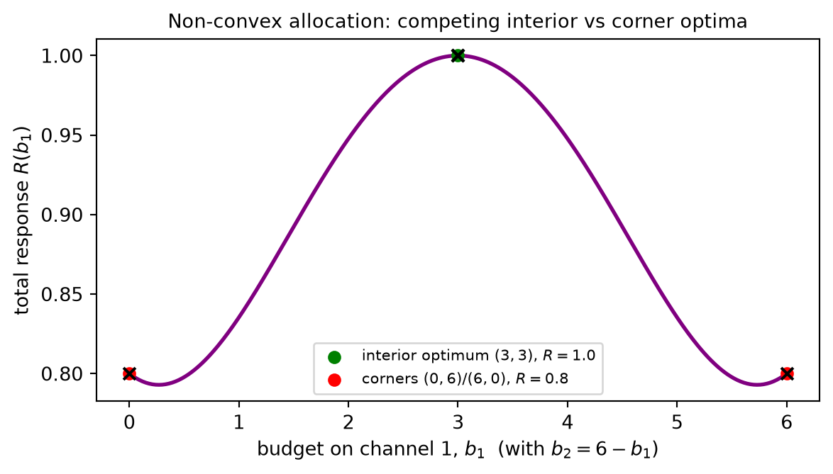
A concrete failure. Take two channels with Hill responses, n = 2, K = 3, and budget B = 6. The symmetric split b = (3, 3) is a stationary point, with total response near 1.0. But the corner allocations b = (6, 0) and b = (0, 6) are also KKT points, each scoring roughly 0.8 — worse than the interior split, yet perfectly valid stationary points of the non-convex problem. A local optimizer started near a corner will converge to that corner and report success, never discovering the better interior allocation. The Code Tie-in below makes this visible, running a multi-start optimizer that lands on different optima depending on where it begins — a direct demonstration that, without convexity, the starting point determines the answer.
What practitioners do. Lacking a global certificate, the working response is threefold. First, run local optimization from multiple starting points and keep the best result found — the multi-start strategy that trades a guarantee for coverage. Second, initialize with domain knowledge, seeding the optimizer near allocations that experience suggests are sensible, so the local search begins in a promising basin. Third, where the structure permits, fit concave surrogate curves or use convex relaxations to bound the achievable response and gauge how far a local solution might be from the true optimum. The intellectually honest position is to report a certified-local optimum and to state plainly that global optimality is not guaranteed — to name the limit of what the method can promise rather than paper over it.
Bridge to the rest of Part IV. This chapter set out the conditions under which optimization is guaranteed to work, and it has now named, just as precisely, when those conditions fail. The two engine chapters that follow are built for the two sides of that divide. Chapter 13 (Linear Programming) studies the fully convex special case in which the feasible set is a polyhedron and the geometry is completely understood — convexity at its most tractable, where the global optimum sits at a vertex and can be found with certainty. Chapter 14 (SLSQP) is the constrained local solver, and it is run from multiple starting points for exactly the reason this rung has laid bare: real response curves are S-shaped, the budget problem is non-convex, and a single descent cannot be trusted to find the global best. The theory of convexity is what tells those algorithms when they have a guarantee and when they are merely doing their honest best — which is precisely the knowledge the next two chapters are built to act on.