Motivation
Part IV and Part V each delivered one half of the budgeting answer. Chapter 12 (Convexity) derived the equal-marginal-returns condition that characterizes an optimal allocation over a concave, saturating channel response, working it by hand to b^\star = (7.2, 1.8) with budget shadow price \lambda = 0.3727 and total response 6.7082; Chapter 13 (Linear Programming) recovered the same allocation as a dual price, reading the shadow price straight off the linear program; and Chapter 14 (SLSQP) reached it a third way, with sequential quadratic programming solving the smooth problem directly and returning the multiplier \lambda as the budget’s shadow price. That trilogy assumed the response curve was a known input — parameters handed over from outside, not estimated from data. Part V removed that assumption. Chapter 15 (the MMM data-generating process) wrote down the probabilistic structure of a realistic campaign, and Chapter 16 (Building & Fitting an MMM) recovered the adstock decay, saturation parameters, and channel coefficients from a synthetic sales series using the inference engine assembled across Chapters 5, 9, and 11. The fitted parameters are not given numbers; they are posterior distributions, uncertain in proportion to what the data could and could not identify. Chapter 18 is the chapter that finally puts both halves together — the chapter a practitioner runs to set next quarter’s spend.
The join raises the chapter’s central question directly: we can solve for the optimal budget, but should we trust the answer? Part IV’s optimizer is exact in the computational sense; given a curve, it finds the allocation that maximizes total response subject to the budget constraint, to any desired tolerance. But the curve it now operates on is the output of an inference procedure, and Chapter 16 showed that typical observational spend data leave the response curve only weakly identified. The Fisher-information geometry of a well-run campaign is not isotropic: some directions in parameter space are tightly pinned by the data, while others are nearly flat. That near-flat direction — the identifiability ridge — runs through the posterior, connecting parameter combinations that agree on historical spend behavior while disagreeing sharply on marginal returns at the counterfactual allocations the optimizer explores. Plugging the posterior mean into the optimizer returns a precise number. The question is whether that precision is warranted.
Two ideas arise in Chapter 18 that have no counterpart in Part IV’s known-curve setting. The first is the shadow price \lambda^\star = dV^\star/dB: the marginal value of an additional budget dollar at the optimum, measuring how fast maximum achievable response increases when the total budget constraint is relaxed. Part IV computed \lambda = 0.3727 as a byproduct of the Lagrangian; this chapter elevates it to the engine of scenario analysis. A practitioner who wants to know what a twenty-percent budget increase buys, or what total budget level is needed to reach a target response, does not need to re-solve the full optimization problem: \lambda^\star answers both questions to first order, and its posterior distribution answers them probabilistically. The second idea is the optimizer’s curse: when the optimizer is applied to an estimated response curve, the point selected by optimization is precisely where estimation noise bent the curve most favorably. The response actually realized at that allocation will on average fall short of the optimizer’s prediction, by an amount equal to the value an experiment that resolved the posterior uncertainty would have delivered. The curse is not a defect of the optimizer; it is an inevitable consequence of selecting from among competing uncertain surfaces the one that looks best.
The chapter’s payoff arc runs in two stages. In the first, plugging the Chapter 16 posterior mean into the Chapter 14 SLSQP solver reproduces Part IV’s exact result: b^\star = (7.2, 1.8), \lambda^\star = 0.3727, total response 6.7082 — closing the loop between the optimization trilogy and the fitted MMM. Against the posterior mean the allocation looks crisp and the confidence appears warranted. In the second stage, the full posterior over response-curve parameters is propagated through the optimizer: for each draw from the Chapter 16 posterior, the solver finds the allocation optimal for that draw, and the resulting distribution of optimal allocations is collected. The identifiability ridge maps, under the optimizer, into a wide distribution of optimal allocations — the point estimate (7.2, 1.8) sits in the middle of a credible region that spans combinations the business would treat as materially different decisions. That gap between the confident allocation the posterior mean implies and the wide allocation the full posterior reveals is the chapter’s wound. It is left open intentionally: the tools to close it are the subject of Part VI, where causal foundations, quasi-experimental designs, and calibration methods make the response curve identifiable in the directions that actually govern budget decisions.
Theory & Proofs
The first three rungs establish the chapter’s analytic spine. Rung 1 states the budgeting problem on a fitted response curve, identifies the key shift that posterior uncertainty introduces, and names the square-root surrogate used for every closed-form result. Rung 2 applies — without re-deriving — the equal-marginal optimality condition from Chapter 12 (Convexity) to recover the Part IV analytic anchor, and observes that the condition holds per posterior draw, inducing a posterior over the optimal allocation. Rung 3 proves the chapter’s keystone identity: the shadow price \lambda^\star reported by the optimizer equals the derivative of the value function with respect to the budget, the identity that turns \lambda^\star into the engine of first-order scenario analysis.
Rung 1 — The budgeting problem on a fitted curve
The goal is to allocate a total budget B across n channels so as to maximise total response:
\max_{b \ge 0,\ \mathbf{1}^\top b = B}\ V(b;\theta) = \sum_{i=1}^n r_i(b_i;\theta_i),
where r_i(b_i;\theta_i) is the fitted MMM response function for channel i — saturating, post-adstock (Chapter 15, the MMM data-generating process), concave and increasing in b_i. The parameter vector \theta collects the adstock decays, saturation curves, and channel coefficients recovered by Chapter 16 (Building & Fitting an MMM). Each r_i is concave in b_i, so V is concave over the budget simplex and the problem has a unique global optimum.
The key shift from Part IV. In Chapters 12, 13, and 14, \theta was a known input: the response curves were given, and the only task was to find the optimal allocation. Chapter 16 removed that assumption. The parameter vector \theta is now the output of an inference procedure and carries a posterior distribution. As a result, the objective V(b;\theta) is random: for a fixed allocation b, different draws from the Chapter 16 posterior yield different total-response surfaces, and the allocation optimal for one draw need not be optimal for another. The optimizer is exact in the computational sense; the surface it operates on is uncertain.
The square-root surrogate. Every closed-form result in this chapter uses the analytically tractable stand-in
r_i(b) = a_i\sqrt{b_i},
with coefficients a = (2,1), budget B = 9, and the shorthand S = \sum_i a_i^2 = 5. Like the true fitted curve, r_i is concave and saturating; unlike it, every number is checkable by hand. The surrogate matches Part IV’s analytic spine exactly, so the numbers (b^\star, \lambda^\star, V^\star) derived below are the same ones Chapters 12, 13, and 14 each reached independently.
Rung 2 — Equal-marginal allocation, applied
The condition. At the optimum, the marginal return of every funded channel must equal the common budget multiplier:
r_i'(b_i^\star) = \lambda^\star \quad \text{for every funded channel } i.
This is the equal-marginal / KKT condition. Its derivation — stationarity of the Lagrangian L(b,\lambda) = V(b) + \lambda(B - \mathbf{1}^\top b) under the concavity of V — appears in Chapter 12 (Convexity), where it was proved both necessary and sufficient for the unique global optimum. It is not re-derived here.
Applying it to the surrogate. The marginal of r_i(b) = a_i\sqrt{b} is r_i'(b) = a_i/(2\sqrt{b}). Setting r_i'(b_i^\star) = \lambda^\star gives
\frac{a_i}{2\sqrt{b_i^\star}} = \lambda^\star \quad\Longrightarrow\quad b_i^\star = \frac{a_i^2}{4(\lambda^\star)^2},
so b_i^\star \propto a_i^2. Summing over channels and applying \sum_i b_i^\star = B determines \lambda^\star:
\sum_i b_i^\star = \frac{S}{4(\lambda^\star)^2} = B \quad\Longrightarrow\quad \lambda^\star = \frac{\sqrt{S}}{2\sqrt{B}},
and substituting back:
b_i^\star = \frac{B\,a_i^2}{S}.
Analytic anchor. With a = (2,1), B = 9, S = 5:
b_1^\star = \frac{9 \cdot 4}{5} = 7.2, \qquad b_2^\star = \frac{9 \cdot 1}{5} = 1.8, \qquad \lambda^\star = \frac{\sqrt{5}}{6} \approx 0.3727,
recovering the allocation that Chapters 12, 13, and 14 each reached by an independent route.
The posterior view. The equal-marginal condition is a statement about the optimum for a specific response curve. When \theta is drawn from the Chapter 16 posterior, the response functions r_i(\cdot;\theta_i) change, and with them the marginals r_i', the optimal allocation b^\star(\theta), and the shadow price \lambda^\star(\theta). The condition holds per posterior draw of \theta: for each draw the optimizer finds a draw-specific allocation and multiplier. Collecting those over all draws produces a posterior distribution over (b^\star, \lambda^\star) — the uncertainty in where and how steeply the value surface peaks, propagated through the optimizer into the budget recommendation.
Rung 3 — Proof P2 (KEYSTONE): the envelope theorem and the shadow price
The shadow price \lambda^\star is not merely an artifact of the Lagrangian; it is the rate at which the maximum achievable response grows as the total budget increases. This identity is the engine of first-order scenario analysis.
Theorem. At the optimum, the marginal value of the budget equals the optimal multiplier:
\frac{dV^\star}{dB} = \lambda^\star.
Proof. Write the value function V^\star(B) = V(b^\star(B)), where b^\star(B) is the optimal allocation as a function of B. Introduce the Lagrangian
L(b,\lambda) = V(b) + \lambda\bigl(B - \mathbf{1}^\top b\bigr).
At the optimum (b^\star,\lambda^\star): (i) the stationarity conditions give \partial L/\partial b_i = r_i'(b_i^\star) - \lambda^\star = 0 for every funded channel i; and (ii) the constraint \mathbf{1}^\top b^\star = B holds, so the constraint term vanishes and V^\star(B) = L(b^\star(B),\lambda^\star(B)). Differentiating L with respect to B by the chain rule:
\begin{aligned}
\frac{dV^\star}{dB}
&= \frac{dL}{dB}\bigg|_{b^\star,\,\lambda^\star} \\[4pt]
&= \sum_i \frac{\partial L}{\partial b_i}\bigg|_\star \frac{db_i^\star}{dB}
+ \frac{\partial L}{\partial \lambda}\bigg|_\star \frac{d\lambda^\star}{dB}
+ \frac{\partial L}{\partial B}\bigg|_\star \\[4pt]
&= \sum_i \bigl(r_i'(b_i^\star) - \lambda^\star\bigr)\frac{db_i^\star}{dB}
+ \bigl(B - \mathbf{1}^\top b^\star\bigr)\frac{d\lambda^\star}{dB}
+ \lambda^\star \\[4pt]
&= \lambda^\star.
\end{aligned}
The \partial L/\partial b_i\big|_\star terms vanish by stationarity and the \partial L/\partial\lambda\big|_\star = B - \mathbf{1}^\top b^\star term vanishes by primal feasibility, so only the explicit B-dependence of L survives: \partial L/\partial B = \lambda^\star. Although b_i^\star changes with B, the response is already maximised over b at the optimum, so first-order perturbations of the allocation induced by a budget change do not alter V to first order — this is the envelope theorem applied to the constrained Lagrangian. \blacksquare
Analytic anchor. Substitute b_i^\star = B\,a_i^2/S into V:
\begin{aligned}
V^\star(B)
&= \sum_i a_i\sqrt{b_i^\star}
= \sum_i a_i\sqrt{\frac{B\,a_i^2}{S}}
= \frac{\sqrt{B}}{\sqrt{S}}\sum_i a_i^2
= \frac{S\sqrt{B}}{\sqrt{S}}
= \sqrt{BS}.
\end{aligned}
So V^\star(B) = \sqrt{BS}, and differentiating:
\frac{dV^\star}{dB} = \frac{\sqrt{S}}{2\sqrt{B}}.
At B = 9, S = 5: dV^\star/dB = \sqrt{5}/6 = \lambda^\star \approx 0.3727. The shadow price the optimizer reports is the budget derivative — not a side product of the Lagrangian algebra but a quantity with a direct economic meaning. A budget increase of \Delta B buys approximately \lambda^\star \cdot \Delta B additional response to first order, and the posterior over \lambda^\star turns that linear approximation into a probability statement. This identity is what the scenario analysis of later rungs will use.
Rung 4 — Propagating curve uncertainty to allocation uncertainty
The equal-marginal analysis of Rung 2 is a statement about one specific response curve: given \theta, it finds the allocation b^\star(\theta) and shadow price \lambda^\star(\theta) that are jointly optimal. When \theta is replaced by the Chapter 16 posterior p(\theta \mid \text{data}), the same analysis applies draw by draw. For each posterior draw \theta^{(s)}, the optimizer finds a draw-specific allocation, multiplier, and peak response:
b^\star\!\left(\theta^{(s)}\right), \quad \lambda^\star\!\left(\theta^{(s)}\right), \quad V^\star\!\left(\theta^{(s)}\right) = \sqrt{S\!\left(\theta^{(s)}\right) B},
where S(\theta^{(s)}) = \sum_i a_i(\theta^{(s)})^2 varies across draws. Collecting these over all posterior samples yields a posterior distribution over the optimal allocation, the shadow price, and the maximum achievable response. The optimizer does not produce one answer; it produces one answer per posterior draw, and the distribution of those answers encodes how much the budgeting decision inherits the parameter uncertainty.
The identifiability ridge amplifies the width. Chapter 16 (Building & Fitting an MMM) showed that the Fisher-information geometry of a typical observational campaign is not isotropic: adstock decay and saturation shape are not separately resolved by spend data that was never designed to move them independently. The resulting near-flat directions in the log-posterior form a ridge — a family of parameter combinations that reproduce historical spend behavior equally well while disagreeing sharply on the marginal returns the optimizer will encounter in the counterfactual spend region. Two draws from opposite sides of the ridge agree on in-sample fit and disagree on where the budget should go; under a correctly propagated posterior, those disagreements become genuine width in the distribution of b^\star(\theta^{(s)}).
The certainty-equivalent plan. A practitioner who plugs the posterior mean \hat\theta into the optimizer obtains the certainty-equivalent (plug-in) allocation:
b^\star_{\text{CE}} = b^\star(\hat\theta).
This is a single, operationally tractable number. It is also a collapse: all the width of the posterior over b^\star(\theta) is discarded in favor of the center, and the resulting allocation is reported with the same confidence one would have if \theta were known. When the ridge is wide, that collapse discards real decision risk — the distribution of b^\star(\theta^{(s)}) spans allocations the business would treat as materially different decisions. Rung 5 makes the cost of that collapse precise.
Rung 5 — Proof P1 (KEYSTONE): the optimizer’s curse
Theorem. For an objective V(b;\theta) with uncertain parameters \theta,
\mathbb{E}_\theta\!\left[\max_b\, V(b;\theta)\right]\ \ge\ \max_b\, \mathbb{E}_\theta\!\left[V(b;\theta)\right].
Proof. Fix any allocation b'. For every realization of \theta, the optimizer is free to choose b', so the maximum is at least as large as the value at b':
\max_b\, V(b;\theta)\ \ge\ V(b';\theta) \qquad \text{for every } \theta.
Taking expectations of both sides preserves the inequality:
\mathbb{E}_\theta\!\left[\max_b\, V(b;\theta)\right]\ \ge\ \mathbb{E}_\theta\!\bigl[V(b';\theta)\bigr].
The left side does not depend on b', so this bound holds uniformly for every choice of b'. In particular it holds when b' is chosen to maximize the right side, giving
\mathbb{E}_\theta\!\left[\max_b\, V(b;\theta)\right]\ \ge\ \max_{b'}\,\mathbb{E}_\theta\!\bigl[V(b';\theta)\bigr]. \quad \blacksquare
No convexity assumption on V in \theta is required; the proof rests only on the trivial pointwise bound that a maximum is at least any particular value. When V(b;\theta) is convex in \theta for each fixed b, Jensen’s inequality gives the same direction from a different route — convexity in \theta is sufficient for the inequality but not necessary.
Three readings.
Over-optimism. Optimizing on a point estimate \hat\theta and reporting \max_b V(b;\hat\theta) is an optimistically biased forecast of the response the chosen plan will actually deliver. The optimizer selects the allocation precisely where the fitted curve looks most favorable, and the fitted curve is most likely to have been bent upward by estimation noise at exactly that point. The response realized out of sample will on average fall short — systematically, not by accident (Smith and Winkler 2006).
Value of information. Re-read the inequality as a gap. The left side is the expected oracle value: what the optimizer could achieve if it ran with full knowledge of \theta before committing to an allocation. The right side is the best expected response achievable by any fixed allocation chosen without knowing \theta. The gap between them is the expected value of perfect information (EVPI): the maximum a decision-maker should pay for an experiment that resolves all uncertainty in \theta before the allocation is set (Gelman et al. 2013).
Bridge to Part VI. The EVPI gap is not uniform across campaigns: it is largest precisely when the Chapter 16 ridge is widest — when observational spend data leave the response curve only weakly identified in the counterfactual spend region the optimizer needs. A confidently-wrong allocation is most costly exactly where the data are least able to adjudicate. The experiments of Part VI — causal foundations, quasi-experimental designs, and calibration — are worth pursuing because they shrink this gap directly, supplying the identification the optimizer requires in the directions the observational data left flat.
Rung 6 — Scenario analysis, made rigorous by the envelope theorem
The Rung 3 identity dV^\star/dB = \lambda^\star converts the shadow price into a practical calculator. Before re-solving the full allocation problem at a perturbed budget B + \Delta B, the envelope theorem supplies the first-order answer:
\Delta V \approx \lambda^\star \cdot \Delta B.
This is exact in the limit \Delta B \to 0 and a useful approximation for moderate perturbations. Re-optimizing at B + \Delta B exposes two sources of departure from the linear prediction. Curvature: because V^\star(B) = \sqrt{SB} is concave, the realized gain falls below the tangent — each successive budget dollar buys less than the previous one, so the linear prediction overestimates the gain for finite \Delta B. Binding caps: when a channel reaches its maximum feasible spend, the active constraint set changes and the shadow price shifts discontinuously — a structural break invisible in the first-order approximation but exposed immediately when the problem is re-solved.
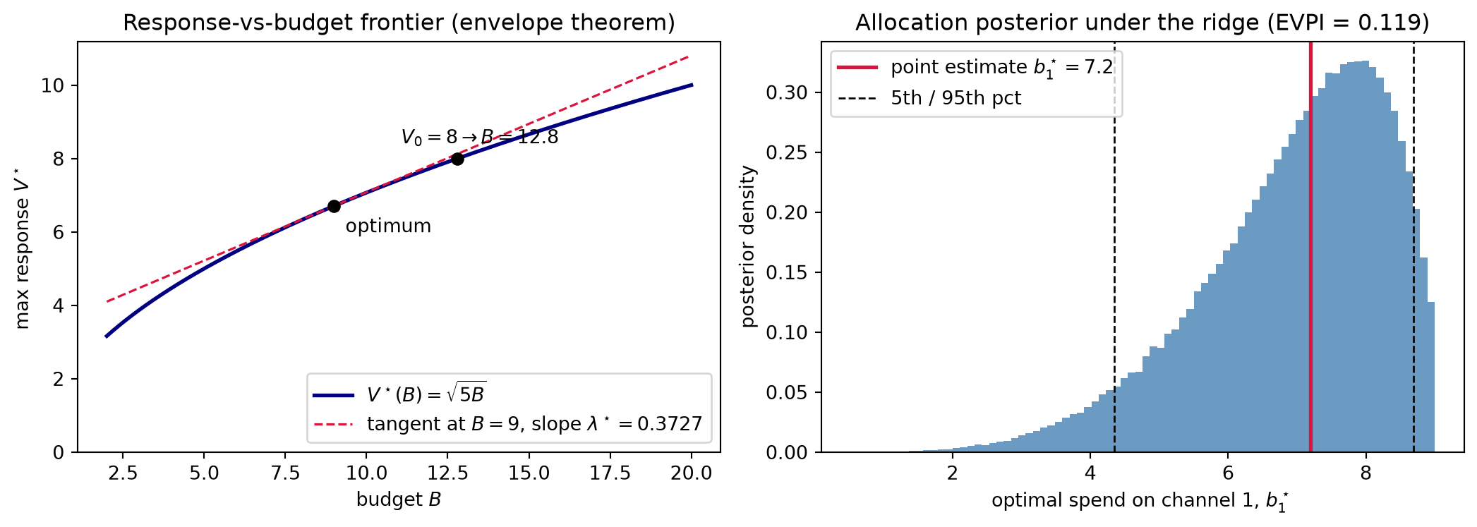
The response-vs-budget frontier. Sweeping B from zero upward traces the value function V^\star(B) = \sqrt{SB} with slope \lambda^\star(B) = \sqrt{S}/(2\sqrt{B}) — the efficiency curve of the campaign. Because V^\star is concave and \lambda^\star is strictly decreasing in B, the frontier visualizes the law of diminishing returns at the portfolio level: the marginal value of budget is highest at low spend and falls as the budget grows. Every budget question — “what does a 20% increase buy?”, “where does the marginal return fall below my hurdle rate?”, “at what budget does the shadow price fall by half?” — is answered by a point on this curve and its slope.
The inverse scenario. The practitioner’s dual question is: what total budget is needed to reach a target response V_0? Since V^\star(B) = \sqrt{SB} is strictly increasing and continuously invertible, inverting the value function gives
V_0 = \sqrt{S B} \quad\Longrightarrow\quad B = \frac{V_0^2}{S},
and the shadow price at that budget is \lambda^\star(B) = \sqrt{S}/(2\sqrt{B}) = S/(2V_0). The frontier and its inverse are the same identity read in two directions: “what does budget B achieve?” and “what budget achieves V_0?” are dual questions, and \lambda^\star is the exchange rate between budget and response in both.
Analytic anchor. To reach target response V_0 = 8 on the a = (2,1) surrogate (S = 5):
B = \frac{8^2}{5} = \frac{64}{5} = 12.8, \qquad \lambda^\star = \frac{5}{2 \cdot 8} = \frac{5}{16} = 0.3125.
Verification: \sqrt{5}/(2\sqrt{12.8}) = 5/16 = 0.3125. \checkmark Compared to the baseline at B = 9 where \lambda^\star \approx 0.3727, the shadow price falls to 0.3125 at B = 12.8 — diminishing returns operating exactly as the concave frontier predicts.
Rung 7 — The wound (closing rung)
Rungs 3 and 6 produce a scenario table that looks crisp and decisive: one value function, one shadow price, one target-budget inversion. That crispness is legitimate when the response curve is known. When the curve comes from the Chapter 16 posterior, the same table is computed per posterior draw and the rows become distributions. Two effects are immediate. First, scenario rankings overlap: the allocation that maximizes response under the posterior mean may rank third under a draw from the identifiability ridge, and the scenario that looks clearly best under \hat\theta may be indistinguishable from the second-best under a plausible alternative. Second, the shadow price carries a wide credible band — the posterior over \lambda^\star(\theta) propagated from parameter uncertainty through the Rung 3 identity — so the first-order answer to “what does \Delta B buy?” is uncertain in proportion to the posterior width in the saturation-coefficient directions.
The deeper concern is the one the Worked Examples in the following section demonstrate directly: two posterior-plausible response curves can produce nearly identical in-sample fit while sending the optimizer to opposite channels. Both curves pass through the historical spend region; they diverge precisely in the counterfactual spend region the optimizer must extrapolate into, and that divergence sends one curve’s optimal allocation heavily toward Channel 1 and the other’s toward a more even split. Good in-sample fit does not imply good budget decisions. The response curve’s identifiability in the counterfactual direction — not its goodness of fit in the historical direction — is what determines whether the optimizer’s prescription can be trusted.
This is the chapter’s wound, and it is structural. Observational MMM identifies the response curve only in the directions the historical spend data excite; the optimizer needs the curve in the counterfactual directions the historical data left flat. The EVPI gap of Rung 5 is positive here not by bad luck but by the geometry of observational campaigns: spend variation reaches the data in the ranges that were historically funded, not in the counterfactual ranges the optimizer explores. The only route to a narrower allocation posterior — a smaller EVPI gap — is to intervene and measure: to move spend deliberately in the directions the observational data left unexcited, generating the identification the optimizer requires.
Part VI opens that route. Chapter 19 (Causal Foundations) supplies the formal framework for distinguishing observational from interventional distributions, making precise in causal-graph language what “the data cannot identify” means and why the identifiability ridge is not a modeling artifact but a structural feature of endogenous spend. Chapter 20 (Quasi-Experimental Designs) shows how geo-experiments, holdout regions, and matched-market tests produce the interventional identification that observational MMM cannot — secants and tangents of the response curve pinned by exogenous spend variation rather than estimated from it. Chapter 21 (Advanced Calibration) uses those identified estimates as likelihood factors that compress the Chapter 16 posterior in the ridge direction, directly narrowing the allocation credible region and shrinking the EVPI gap. The wound this chapter names is the gap those three chapters close. This is the wound that ends Part V.
Worked Examples
Three worked examples carry the chapter’s main results into arithmetic — the first closing the Part IV loop by recovering the exact allocation the three optimization chapters each found by an independent route, the second building a scenario table driven by the shadow price and tracing the response frontier to its inverse, and the third making the optimizer’s curse and the identifiability wound concrete with numbers.
WE1 — Closing the Part IV loop
Setup.
Square-root surrogate r_i(b) = a_i\sqrt{b_i} with a = (2,1), budget B = 9, S = \sum_i a_i^2 = 5.
Equal-marginal allocation.
Applying the Rung 2 closed-form directly:
b_1^\star = \frac{B\,a_1^2}{S} = \frac{9 \cdot 4}{5} = 7.2, \qquad b_2^\star = \frac{B\,a_2^2}{S} = \frac{9 \cdot 1}{5} = 1.8.
Verifying equal marginals.
Computing r_i'(b_i^\star) = a_i/(2\sqrt{b_i^\star}) at each channel:
r_1'\!(7.2) = \frac{2}{2\sqrt{7.2}} = \frac{1}{\sqrt{7.2}} \approx 0.3727, \qquad r_2'\!(1.8) = \frac{1}{2\sqrt{1.8}} \approx 0.3727.
Both equal the Rung 2 formula \lambda^\star = \sqrt{S}/(2\sqrt{B}) = \sqrt{5}/6 \approx 0.3727. The equal-marginal condition holds at both channels; the KKT conditions are satisfied and the optimum is confirmed.
Total response.
V^\star = 2\sqrt{7.2} + \sqrt{1.8} = 2(2.6833) + 1.3416 = 6.7082 = \sqrt{45}.
Envelope-theorem check.
The Rung 3 proof established V^\star(B) = \sqrt{SB}. Evaluating and differentiating at B = 9:
V^\star(9) = \sqrt{5 \cdot 9} = \sqrt{45} = 6.7082, \qquad \left.\frac{dV^\star}{dB}\right|_{B=9} = \frac{\sqrt{5}}{2\sqrt{9}} = \frac{\sqrt{5}}{6} \approx 0.3727 = \lambda^\star.
The derivative of the value function with respect to budget equals the Lagrange multiplier: the envelope theorem, made arithmetic.
The loop closes.
The numbers b^\star = (7.2, 1.8), \lambda^\star \approx 0.3727, and V^\star = 6.7082 first appeared in Chapter 12’s Lagrangian analysis, reappeared as the dual price of Chapter 13’s linear program, and surfaced a third time as the SLSQP multiplier in Chapter 14. They appear here a fourth time, now as the output of the fitted-curve optimizer applied to the Chapter 16 surrogate at its posterior mean. Part IV assumed the response curve was a known input; Part V estimated it from data. This is where the Part IV loop closes.
WE2 — Scenario analysis via the shadow price
Setup.
Same surrogate and baseline optimum as WE1: B = 9, b^\star = (7.2, 1.8), \lambda^\star \approx 0.3727, V^\star = 6.7082. The Rung 6 first-order predictor is \Delta V \approx \lambda^\star \cdot \Delta B.
Scenario table.
| Baseline |
B = 9 |
6.71 |
— |
— |
| +20\% |
B = 10.8 |
\sqrt{54} = 7.35 |
6.71 + 0.37\cdot 1.8 = 7.38 |
+0.03 |
| -20\% |
B = 7.2 |
\sqrt{36} = 6.00 |
6.71 - 0.37\cdot 1.8 = 6.04 |
+0.04 |
| Cap b_1 \le 5 |
b = (5,\,4) |
2\sqrt{5}+2 = 6.47 |
n/a |
Cap binds |
| Ch. 2 dark |
b = (9,\,0) |
2\sqrt{9} = 6.00 |
n/a |
Struct. change |
In the budget-shift rows, the shadow price gives a no-re-solve answer: multiply \lambda^\star = 0.3727 by the budget change and add to the baseline. The prediction overshoots in both directions — 7.38 versus realized 7.35 for an increase, and 6.04 versus realized 6.00 for a decrease. Because V^\star(B) = \sqrt{5B} is concave, the tangent at B = 9 lies above the curve at every other budget; the first-order prediction is an optimistic upper bound for any finite |\Delta B|, and the overshoot grows with (\Delta B)^2.
The cap and dark rows cannot be addressed by the single shadow price: both alter the active constraint set. Under the cap b_1 \le 5, the 2.2 budget units the optimizer would have directed to channel 1 spill to channel 2 (b_2 = 4), but binding the more efficient channel costs 6.7082 - 6.4721 = 0.2361 units of response — a structural loss invisible in the first-order predictor. With channel 2 dark, V = 2\sqrt{9} = 6.0000: a 10.6\% loss relative to the unconstrained optimum, coinciding with the -20\% budget row by a feature of the surrogate’s parameters.
The response frontier and its inverse.
Sweeping B traces the value function and its slope — the campaign’s efficiency curve:
V^\star(B) = \sqrt{5B}, \qquad \lambda^\star(B) = \frac{\sqrt{5}}{2\sqrt{B}}.
Both are plotted in the Code Tie-in. As B grows, V^\star rises at a declining rate and \lambda^\star falls, the law of diminishing returns visible in the slope. The inverse answers “what budget achieves target response V_0 = 8?” Inverting V^\star(B) = \sqrt{5B} and specializing to V_0 = 8, S = 5:
B = \frac{V_0^2}{S} = \frac{64}{5} = 12.8, \qquad \lambda^\star(12.8) = \frac{S}{2V_0} = \frac{5}{16} = 0.3125.
Verification: \sqrt{5 \times 12.8} = \sqrt{64} = 8. \checkmark The shadow price at the required budget, 0.3125, is below the baseline 0.3727: pushing response from 6.7082 to 8.0000 requires spending into a region of further diminishing returns, exactly as the concave frontier predicts.
WE3 — The wound
Three parts: a posterior over the optimal allocation, the optimizer’s curse in numbers, and two equally-fitted curves that send the optimizer to opposite channels.
WE3(a) — The allocation posterior.
The Chapter 16 ridge leaves the attribution split poorly identified. Represent this with a joint posterior on a = (a_1, a_2) that pins the total-response direction (1,1) tightly — the level of response is well identified by the sales series — while placing wide mass on the split direction (1,-1), reflecting near-flat Fisher information in that direction. For each posterior draw a^{(s)}, the closed-form equal-marginal rule gives the draw-specific optimal allocation:
b_1^\star\!\left(a^{(s)}\right) = \frac{B\,\bigl(a_1^{(s)}\bigr)^2}{\bigl(a_1^{(s)}\bigr)^2 + \bigl(a_2^{(s)}\bigr)^2}.
Propagating a representative posterior — seeded computation in the Code Tie-in — the distribution of b_1^\star has median \approx 7.2 but a 5th–95th percentile band of approximately [4.35,\,8.69]: more than four budget units out of a total of nine. The confident point estimate 7.2 is one draw in a wide distribution. Every allocation in that band is equally consistent with the historical sales data; the draws disagree only in the counterfactual spend region the optimizer must extrapolate into.
WE3(b) — The optimizer’s curse, numerically.
The practitioner who optimizes on the posterior-mean curve a = (2,1), S = 5 achieves
\max_b\,\mathbb{E}_a\!\left[V(b;\,a)\right] = \sqrt{S \cdot B} = \sqrt{5 \cdot 9} = 6.7082.
An oracle who knows each posterior draw’s curve before committing to an allocation achieves
\mathbb{E}_a\!\left[\max_b V(b;\,a)\right] = \sqrt{B}\,\mathbb{E}_a\!\left[\|a\|\right] \approx 6.8276.
The gap 6.8276 - 6.7082 \approx 0.1194 \ge 0 is the optimizer’s curse in numbers. The allocation chosen from the estimated curve falls short of the oracle by \approx 0.12 response units — roughly 1.8\% of total response. Rung 5 proved this gap is non-negative for any uncertain objective; here it equals the EVPI: the maximum value of an experiment that resolved the Chapter 16 ridge before the budget decision is made.
WE3(c) — Identical fit, opposite allocations.
Place two response curves on the circle \|a\|^2 = S_0 = 5.0625, so both achieve the same maximum achievable response
V^\star = \sqrt{B \cdot S_0} = \sqrt{9 \times 5.0625} = 6.75
exactly. Parameterize by angle \theta:
a(\theta) = \bigl(\sqrt{S_0}\cos\theta,\; \sqrt{S_0}\sin\theta\bigr) = (2.25\cos\theta,\; 2.25\sin\theta).
At \theta = 15^\circ (channel 1 dominant), a \approx (2.173,\,0.582) and a_1^2 \approx 4.722, a_2^2 \approx 0.339. The optimal allocation is
b^\star \approx \left(\frac{9 \times 4.722}{5.0625},\; \frac{9 \times 0.339}{5.0625}\right) \approx (8.40,\; 0.60).
At \theta = 75^\circ (channel 2 dominant), a \approx (0.582,\,2.173): the roles of a_1 and a_2 exchange by symmetry, giving b^\star \approx (0.60,\,8.40).
| \theta = 15^\circ |
2.173 |
0.582 |
6.75 |
8.40 |
0.60 |
| \theta = 75^\circ |
0.582 |
2.173 |
6.75 |
0.60 |
8.40 |
The two curves differ along the contrast direction (1,-1) — exactly the direction the Chapter 16 ridge leaves unidentified — so at a balanced historical spend mix they reproduce the sales series equally well, since the in-sample fit depends on a only through a_1\sqrt{b_1^{\text{hist}}} + a_2\sqrt{b_2^{\text{hist}}} \propto a_1 + a_2, which is identical for the two mirror-image curves. The data cannot tell them apart. Fixing \|a\| equal (the circle) makes their maximum achievable response identical too, 6.75, isolating the allocation as the only thing that differs — and it differs maximally: the optimal split depends on the ratio a_1^2 : a_2^2, which inverts between the curves, so one sends 93\% of the budget to channel 1 and the other 93\% to channel 2. A model-selection exercise that chooses between them by goodness of fit alone cannot distinguish them, yet the implied budget decisions are as far apart as they could be.
Good fit does not imply good decisions. The response curve’s identifiability in the counterfactual direction — the direction the optimizer must extrapolate into — is what determines whether the allocation can be trusted. This is the wound Rung 7 named, and it is left open intentionally: the tools to close it are the subject of Part VI.
Exercises
C – Conceptual / Reading Comprehension
C1. A colleague reports that the budget optimizer, run on the fitted MMM, predicts a total response of 6.83 at its chosen allocation, and proposes to commit to that number in next quarter’s plan. Using the optimizer’s curse, explain why 6.83 is an optimistically biased forecast of the response the plan will actually realize, and what the honest forecast should be anchored to instead.
C2. Define the expected value of perfect information (EVPI) in the budgeting context, and explain operationally why running an experiment shrinks it. Why does the EVPI gap depend on which directions of the response curve the data leaves unidentified, rather than on the overall goodness of fit?
C3. Two candidate response curves achieve identical in-sample fit but send the optimizer’s budget to opposite channels. Explain why “pick the better-fitting model” cannot resolve the disagreement, and identify what kind of additional information would. Connect your answer to why Part V ends on a wound that Part VI is needed to heal.
C4. The shadow price \lambda^\star falls from 0.3727 at B = 9 to 0.3125 at B = 12.8. State what \lambda^\star measures, and explain why its decline is the law of diminishing returns expressed at the portfolio level.
B – By Hand
Use the square-root surrogate r_i(b) = a_i\sqrt{b_i} with a = (2, 1), so S = \sum_i a_i^2 = 5.
B1. Starting from the equal-marginal allocation b_i^\star = B a_i^2/S, derive the closed-form value function V^\star(B) = \sqrt{SB}. Hence confirm the envelope identity dV^\star/dB = \lambda^\star = \sqrt{S}/(2\sqrt{B}), and evaluate both at B = 9.
B2. Compute the first-order shadow-price prediction of the total response at a 20\% budget increase (B = 10.8) and compare it to the exact V^\star(10.8). Is the prediction an over- or under-estimate? Explain the sign from the concavity of V^\star.
B3. Solve the inverse scenario: find the budget B required to reach a target response V_0 = 8, and read off the shadow price at that budget. Confirm B = 12.8 and \lambda^\star = 5/16.
B4. Impose the cap b_1 \le 5. Show that the cap binds, find the constrained optimum (b_1, b_2) and its total response, and quantify the response lost relative to the uncapped optimum 6.7082.
P – Prove It
P1. Prove the optimizer’s curse: for any objective V(b;\theta) with random \theta,
\mathbb{E}_\theta\!\left[\max_b V(b;\theta)\right] \ge \max_b \mathbb{E}_\theta\!\left[V(b;\theta)\right].
Your proof should rest only on the pointwise bound that a maximum is at least any particular value; state clearly where that bound enters and why no convexity assumption on V in \theta is required.
P2. Prove the envelope theorem for the equality-constrained budget problem: with Lagrangian L(b,\lambda) = V(b) + \lambda(B - \mathbf{1}^\top b) and optimum (b^\star(B), \lambda^\star(B)), show dV^\star/dB = \lambda^\star. Account explicitly for the dependence of both b^\star and \lambda^\star on B, and identify which terms vanish and why.
P3. Let \theta have mean \bar\theta and suppose V(b;\theta) is convex in \theta for each fixed b. Show that the certainty-equivalent value \max_b V(b;\bar\theta) is a lower bound for the oracle value \mathbb{E}_\theta[\max_b V(b;\theta)], and explain how this relates to the optimizer’s curse of P1. (Hint: combine Jensen’s inequality with the result of P1.)
A – Applied / Code
A1. Modify the Code Tie-in’s ridge posterior by widening the poorly-identified contrast direction (increase the coefficient 0.45 on the (1,-1) component). Show that both the optimizer’s-curse gap \mathbb{E}[\max] - \max\mathbb{E} and the width of the b_1^\star posterior band grow as the ridge flattens. Plot the EVPI gap as a function of the contrast standard deviation.
A2. Add a minimum-spend floor b_i \ge f (e.g. f = 2) to the budget problem and re-solve with SLSQP. Report the constrained optimum and recover the floor’s shadow price as the multiplier on the active floor constraint — the response gained per unit the floor is relaxed. Interpret the sign.
A3. Extend the optimizer to three channels with coefficients a = (2, 1.5, 1) and budget B = 12. Solve for the optimal allocation and shadow price with SLSQP, verify the equal-marginal condition holds across all three funded channels, and confirm the closed-form V^\star(B) = \sqrt{SB} with S = \sum_i a_i^2.