Motivation
Chapter 15 ran the MMM machine forward: it wrote down the data-generating process, assembled the adstock and saturation transforms into a structural equation, proved the properties of each component, and then ran the whole pipeline in simulation — producing a synthetic two-year weekly sales series from a known parameter vector. That chapter ended on an identification wound: you cannot recover the response curve from observational spend alone, because operating-range confinement, channel collinearity, and baseline confounding conspire to make the inverse problem ill-posed. This chapter takes the wound as its starting point. Given only the observed spend and the synthetic sales that Chapter 15 generated, the task is to run the machine backward and recover the adstock decay, saturation half-point, shape exponent, and channel scales that produced them. That is the inverse problem, and this chapter shows how Bayesian inference solves it — partially, honestly, and with explicit uncertainty about what the data cannot tell us.
The solution draws on every tool the book has built. The structural equation from Chapter 15 supplies the likelihood: it tells us exactly what probability distribution over sales the model assigns to each candidate parameter vector. Chapter 5’s treatment of priors and the maximum a posteriori principle supplies the regularization that carries the load on the directions the likelihood cannot pin. Chapters 9 and 10 supply the sampler — Hamiltonian Monte Carlo via NUTS — that explores the posterior without requiring its closed form, navigating the curved, high-dimensional geometry of the adstock–saturation parameter space. Chapter 11 supplies the diagnostics: \hat{R}, effective sample size, and posterior predictive checks that tell us whether the chains have converged and whether the fitted model generates data that resembles the observed series. There is little new theory here. This is the chapter the preface promised: the integration of the preceding machinery into a single, end-to-end Bayesian MMM, one whose moving parts are already in place and whose novelty lies in the way they compose.
Working on synthetic data is a deliberate choice, and the advantage it provides is a precise definition of success. In a real campaign, “success” is ambiguous: a model that fits the in-sample sales series beautifully might have the wrong saturation curve, the wrong attribution, the wrong adstock decay — and the real data cannot tell us, because we do not know the truth. The synthetic series from Chapter 15 does. Because every parameter in the data-generating process is on record, we can ask not merely whether the model fits but whether it recovers the parameters that generated the data. A posterior whose mean lies near the true value and whose width reflects the actual uncertainty in the available data is a success; a posterior that fits the series but concentrates on the wrong parameter vector is not, regardless of how small its residuals are. This distinction — fit versus recovery — is the discipline synthetic data imposes, and it is the criterion this chapter applies to evaluate the inference.
The tension from Chapter 15’s wound runs through everything that follows. When spend varies across a meaningful range of the saturation curve, the likelihood surface is informative and the posterior concentrates near the true parameters; recovery succeeds. When spend is confined to a narrow operating range — as it will be for one of the chapter’s channels — the likelihood is nearly flat along a ridge in the (\beta, K) plane, and the posterior is wide in those directions, reflecting genuine uncertainty rather than a failure of the sampler. This is not a defect to be corrected; it is the correct Bayesian answer to an underdetermined question. Priors carry the load on those unidentified directions, and the chapter shows how the choice of prior scale shapes the posterior without overriding the data’s verdict where the data are informative. That failure mode — tight posteriors for some parameters, prior-dominated for others — is the precise setting that motivates Part VI, where experimentally induced spend variation finally breaks the degeneracy.
Theory & Proofs
The theory develops in three rungs. Rung 1 translates Chapter 15’s structural equation directly into a Gaussian likelihood, identifies the mean function, and contrasts the nonlinear role of (K, n, \lambda) here with the linear case of Chapter 5. A short proposition then establishes the non-conjugacy of this likelihood — the formal obstruction that forces approximate or sampling-based inference. Rung 2 specifies weakly informative priors that encode domain knowledge and carry the regularization load on the directions the likelihood cannot pin.
Rung 1 — From DGP to likelihood
Chapter 15’s generative model runs forward: a parameter vector \theta = (\beta, K, n, \lambda, \ldots) produces a mean trajectory through the adstock–saturation pipeline, and Gaussian noise is added on top. Bayesian inference runs the same model backward. The key observation is that the noise model — already specified in Chapter 15’s structural equation — supplies a Gaussian likelihood directly.
Collect the baseline terms into a single function \text{baseline}_t — absorbing the intercept, trend, seasonality, and any controls — so that the mean function is
\mu_t(\theta) = \text{baseline}_t + \sum_{i=1}^{C} \beta_i\, g\!\big(a_\lambda(x_{i,t});\, K_i,\, n_i\big).
The noise term \varepsilon_t \sim \mathcal{N}(0, \sigma^2) from Rung 1 of Chapter 15 then determines the observation model: each week’s sales is Gaussian around its mean,
y_t \mid \theta \;\sim\; \mathcal{N}\!\big(\mu_t(\theta),\, \sigma^2\big), \qquad t = 1, \ldots, T.
Assuming conditional independence across weeks, the joint log-likelihood factors into a sum over time:
\ell(\theta) = -\frac{1}{2\sigma^2}\sum_{t=1}^{T} \big(y_t - \mu_t(\theta)\big)^2 - T\log\sigma + \text{const}.
Contrast with Chapter 5. In the Bayesian linear regression of Chapter 5 the mean function was \mu_t = X_t^\top \beta — linear in the parameters — and the likelihood was a Gaussian in \beta that could be analyzed in closed form. Here \mu_t(\theta) is nonlinear in (K_i, n_i, \lambda_i): the Hill function g(a;\, K, n) = a^n / (K^n + a^n) is a rational power function of (K, n), and the adstock a_\lambda(x)_t = \sum_{k=0}^{\infty} \lambda^k x_{t-k} is a weighted sum whose weights are powers of \lambda. That nonlinearity breaks the conjugate structure and makes the posterior intractable — as the proposition below establishes.
Proposition — Non-conjugacy
Proposition (Non-conjugacy). The posterior p(\theta \mid y_{1:T}) has no closed form: no standard conjugate prior family closes the Gaussian likelihood of Rung 1 under multiplication.
Proof (sketch). Conjugacy requires that the prior and likelihood share a functional form such that their product is the kernel of a distribution from the same family. For parameters entering the likelihood linearly — such as \beta_i in the large-K limit where g \approx x/K is nearly linear — a Gaussian or half-normal prior on \beta_i closes under the Gaussian likelihood, yielding a Gaussian posterior. The closure fails for (K_i, n_i, \lambda_i). The likelihood’s dependence on these parameters enters through g(a_\lambda(x_{i,t});\, K_i, n_i) = a_\lambda(x_{i,t})^{n_i}/(K_i^{n_i} + a_\lambda(x_{i,t})^{n_i}) — a rational power function — and through the adstock weights \lambda_i^k, powers of \lambda_i summed over all lags. Multiplying the Gaussian likelihood by any standard prior on (K_i, n_i, \lambda_i) — Beta, Gamma, half-normal, log-normal — does not produce the kernel of a recognized distribution: no functional identity collapses the product into a named family, and the normalizing constant \int p(y_{1:T} \mid \theta)\, p(\theta)\, d\theta has no closed-form expression. We must therefore either approximate the posterior (MAP estimation combined with a Laplace approximation around the mode) or sample it directly (MCMC). The remainder of this chapter uses the latter. \blacksquare
Rung 2 — Priors
Because the likelihood cannot identify all of \theta — the wound from Chapter 15 runs straight through the posterior — the choice of prior is not cosmetic: it is load-bearing. A prior encodes domain knowledge about plausible parameter values and regularizes the posterior in the directions the likelihood cannot pin. The guiding principle is weakly informative: the prior should exclude physically impossible or economically absurd values without forcing the posterior away from what the data actually say.
Adstock decay \lambda_i \sim \text{Beta}(2, 2). The decay parameter lives on [0, 1) by definition. A \text{Beta}(2, 2) distribution is symmetric around 0.5, placing mass in the interior and ruling out both zero carryover (\lambda = 0, no memory at all) and near-permanent memory (\lambda \to 1), while remaining diffuse enough to move toward the data’s verdict. If category-level evidence suggests shorter or longer carryover, the Beta’s two shape parameters can encode that asymmetry.
Half-saturation point K_i \sim \text{HalfNormal}(\sigma_K). The half-saturation point is strictly positive — it is a spend level. A half-normal prior places mass on (0, \infty) with a single scale parameter. The scale \sigma_K should be set to the order of magnitude of the observed spend distribution for channel i: if typical weekly spend runs in the hundreds of thousands, a matching \sigma_K keeps the prior from anchoring far from realistic values.
Shape exponent n_i \sim \text{HalfNormal}(\sigma_n). The shape exponent is positive by the Hill function’s definition, and empirical marketing saturations rarely exhibit very large shape parameters. A half-normal with scale \sigma_n \approx 1 places prior mass near the range 1–2 — covering pure concavity (n \le 1) and mild S-shape (n \approx 2) — while permitting larger values if the data support a pronounced convex toe.
Channel scale \beta_i \sim \text{HalfNormal}(\sigma_\beta). Channel coefficients are non-negative: advertising raises sales or has no effect, but does not reduce them. A half-normal encodes this sign constraint while remaining diffuse over the plausible range of revenue per unit of saturated exposure.
Noise scale \sigma \sim \text{HalfNormal}(\sigma_0). The observation noise is a standard deviation and therefore positive. A half-normal prior on \sigma is weakly informative and guards against posteriors that collapse \sigma toward zero — a pathology that can arise when a flexible mean function overfits in-sample.
Throughline to Proof P2. Together, these priors ensure that the posterior p(\theta \mid y_{1:T}) is proper even when the likelihood is nearly flat along the identification ridge from Chapter 15. Proof P2 (later in this chapter) will make this precise: when the data are weak — when spend is confined to a narrow operating range — the likelihood supplies almost no curvature in the (K_i, \beta_i) direction, and the half-normal priors on K_i and \beta_i provide the missing regularization, keeping the posterior concentrated without overriding the data’s verdict where the data are informative. The prior is the correct Bayesian formalization of the domain knowledge that advertising effects are positive, bounded, and measured on scales the practitioner can calibrate before seeing the data.
Rung 3 — Posterior geometry and sampling
The identification ridge that Chapter 15 traced in parameter space does not vanish when we condition on data; it reappears as strong posterior correlation between \beta and K. Along the ridge, many (\beta, K) pairs produce nearly identical trajectories, so the posterior assigns non-negligible probability to a curved, elongated region rather than a tight ellipsoid. In the confined-spend case — where all observations cluster near a single operating point x_0 — the ridge becomes a nearly flat direction in the posterior: moving along it changes the likelihood so little that the prior alone provides the restoring force. This geometry, characterized by strong curvature in some directions and near-flatness in others, is ill-conditioned in the sense that the Hessian of the log-posterior has a large condition number, and it is precisely the setting gradient-based samplers are designed to handle. NUTS (Chapter 10) adapts its step size and trajectory length to the local curvature of the log-posterior, leaning into the elongated geometry and exploring it efficiently; divergences (Chapter 11) flag the points where a fixed step size fails — where the trajectory overshoots the ridge and the sampler’s acceptance rate collapses. Rather than re-derive those mechanics here, the chapter demonstrates the geometry concretely: the MAP estimate locates the posterior mode, the Hessian of the log-posterior at the mode gives a Laplace approximation that makes the ill-conditioning visible as a numerical matrix, and a Metropolis sampler run on the same posterior shows the chains tracing the ridge directly.
Proof P1 — Local identifiability via Fisher information
Proposition P1. For the model y_t \sim \mathcal{N}(\mu_t(\theta), \sigma^2) (independent across t), the parameter \theta is locally identified at \theta_0 if and only if the Fisher information matrix
I(\theta_0) = \frac{1}{\sigma^2}\sum_{t=1}^{T} \nabla_\theta\mu_t(\theta_0)\,\nabla_\theta\mu_t(\theta_0)^\top
is nonsingular.
Proof. We work through four steps: derive the Fisher information for this model; show that singularity of I(\theta_0) is equivalent to the existence of a direction along which the likelihood is flat; apply that equivalence to the MMM mean function; and read off the answer to Chapter 15’s open question.
Step 1 — Deriving the Fisher information. The joint log-likelihood, under independence across t, is
\ell(\theta) = -\frac{1}{2\sigma^2}\sum_{t=1}^{T}\big(y_t - \mu_t(\theta)\big)^2 + \text{const}.
Differentiating with respect to \theta gives the score vector
\nabla_\theta\ell = \frac{1}{\sigma^2}\sum_{t=1}^{T}\big(y_t - \mu_t(\theta)\big)\,\nabla_\theta\mu_t(\theta).
Differentiating again yields the Hessian
\nabla^2_\theta\ell = \frac{1}{\sigma^2}\sum_{t=1}^{T}\Big[(y_t - \mu_t(\theta))\,\nabla^2_\theta\mu_t(\theta) - \nabla_\theta\mu_t(\theta)\,\nabla_\theta\mu_t(\theta)^\top\Big].
The Fisher information is defined as I(\theta) = -\mathbb{E}_\theta[\nabla^2_\theta\ell]. Under the model, \mathbb{E}_\theta[y_t - \mu_t(\theta)] = 0 for each t, so the first term inside the sum vanishes in expectation, and
I(\theta) = \frac{1}{\sigma^2}\sum_{t=1}^{T} \nabla_\theta\mu_t(\theta)\,\nabla_\theta\mu_t(\theta)^\top.
This is a sum of rank-one outer products; its rank equals the dimension of the span of \{\nabla_\theta\mu_t(\theta)\}_{t=1}^T.
Step 2 — Singular I(\theta_0) if and only if a likelihood-flat direction exists. Suppose I(\theta_0) is singular. Choose a nonzero vector d in its null space, so I(\theta_0)\,d = 0. Then
0 = d^\top I(\theta_0)\, d = \frac{1}{\sigma^2}\sum_{t=1}^{T}\big(\nabla_\theta\mu_t(\theta_0)^\top d\big)^2.
This is a sum of non-negative squares equal to zero, so each term must vanish: \nabla_\theta\mu_t(\theta_0)^\top d = 0 for every t = 1, \ldots, T. By the chain rule, displacing \theta from \theta_0 by a small step \epsilon d changes each mean function to first order by \mu_t(\theta_0 + \epsilon d) = \mu_t(\theta_0) + \epsilon\,\nabla_\theta\mu_t(\theta_0)^\top d + O(\epsilon^2) = \mu_t(\theta_0) + O(\epsilon^2). The mean trajectory is therefore unchanged to first order, the log-likelihood is unchanged to first order, and the direction d is a likelihood-flat direction at \theta_0: moving along d leaves the data distribution unaltered, so \theta_0 is not locally identified. Conversely, if I(\theta_0) is nonsingular, its null space is trivial and no such direction d exists. For every nonzero d, the quadratic form d^\top I(\theta_0)\, d > 0, which means at least one term (\nabla_\theta\mu_t^\top d)^2 > 0: some mean \mu_t is sensitive to displacement along d. The log-likelihood is therefore strictly curved in every direction at \theta_0, and \theta_0 is locally identified.
Step 3 — Application to the MMM. The mean function \mu_t(\theta) = \text{baseline}_t + \sum_i \beta_i\, g(a_\lambda(x_{i,t});\, K_i, n_i) passes spend through the adstock operator a_\lambda and the Hill saturation g, so each component of \nabla_\theta\mu_t depends on the operating point x_t at time t. If all spend observations are confined to a single value x_0 — so that x_t = x_0 for all t — then every gradient \nabla_\theta\mu_t equals the same vector v = \nabla_\theta\mu(\theta_0;\, x_0). The information matrix collapses to
I(\theta_0) = \frac{T}{\sigma^2}\, v\, v^\top,
which has rank 1 < \dim\theta: it is singular. This is the information-matrix restatement of Chapter 15’s Proof P4: the flat ridge in the (\beta, K) plane is exactly the null space of v\, v^\top, populated by all directions orthogonal to v.
When spend instead spans a range of operating points, the gradient vectors \{\nabla_\theta\mu_t\}_{t=1}^T vary with t. If they collectively span the full parameter space \mathbb{R}^{\dim\theta}, then I(\theta_0) has full rank by the outer-product construction in Step 1, and \theta_0 is locally identified.
Step 4 — Answering Chapter 15’s open question. Chapter 15 closed with the question: how much spend variation is enough? The Fisher information matrix gives a crisp answer. Spend variation is sufficient for local identifiability if and only if the resulting gradient vectors \{\nabla_\theta\mu_t(\theta_0)\}_{t=1}^T span the parameter space — equivalently, if I(\theta_0) is nonsingular. For the two-parameter slice (\beta, K) of the worked example to follow, this means at least two time points whose spending levels produce non-parallel gradient vectors: two distinct operating points on the Hill curve whose tangent directions in (\beta, K)-space are linearly independent. One operating point is always insufficient, because it yields a rank-one I(\theta_0); two generic operating points generically suffice. \blacksquare
Rung 4 — The fitting workflow
Bayesian inference for the MMM follows five stages in disciplined sequence, each catching a distinct failure mode before the next stage begins.
(1) Prior predictive check. Draw \theta \sim p(\theta), pass each draw through the mean function \mu_t(\theta), and simulate a sales series; the distribution of simulated series should look plausible — bounded, seasonal, in the right order of magnitude — before any observed data enter the analysis.
(2) Fit. Condition on y_{1:T} and locate the posterior p(\theta \mid y_{1:T}), either by finding the MAP mode and forming a Laplace approximation around it, or by running a gradient-based sampler (Chapters 9–10) to draw directly from the posterior.
(3) Convergence diagnostics. Inspect \hat{R}, effective sample size, and divergence counts for each parameter (Chapter 11); values of \hat{R} > 1.01, low effective sample sizes, or any divergences signal that the chains have not mixed and the draws do not faithfully represent p(\theta \mid y_{1:T}).
(4) Posterior predictive check. Draw replicated series y^{\text{rep}}_{1:T} by sampling \theta from the posterior and simulating forward; compare them to the observed series to test whether the fitted model reproduces the scale, seasonality, and autocorrelation structure of the data, or whether a systematic discrepancy reveals model misspecification.
(5) Parameter recovery. Because the data are synthetic and the true \theta is on record, compare each marginal posterior to its ground-truth value; a 90% credible interval that contains the true value constitutes recovery, and a posterior that fits the series but concentrates on the wrong parameter vector signals the identification wound.
Proof P2 — Prior dominates the unidentified ridge
Proposition P2. Suppose the log-likelihood is flat along a direction d at \theta_0: \ell(\theta_0 + s\,d) = \ell(\theta_0) for all s in a neighborhood of 0. Then along that ridge the posterior is proportional to the prior: p(\theta_0 + s\,d \mid y) \propto p(\theta_0 + s\,d), and the conditional posterior density of s is the prior restricted to the ridge.
Proof. Define L_0 := e^{\ell(\theta_0)}. By assumption,
L(\theta_0 + s\,d) = e^{\ell(\theta_0 + s\,d)} = e^{\ell(\theta_0)} = L_0
for all s in the neighborhood. Bayes’ theorem gives p(\theta \mid y) \propto p(\theta)\,L(\theta). Restricting to the ridge \theta = \theta_0 + s\,d,
p(\theta_0 + s\,d \mid y) \propto p(\theta_0 + s\,d)\,L(\theta_0 + s\,d) = p(\theta_0 + s\,d)\,L_0 \propto p(\theta_0 + s\,d),
since L_0 does not depend on s. Normalizing along the ridge yields the conditional density of s given that \theta lies on the ridge:
p(s \mid \theta \in \text{ridge},\, y) = \frac{p(\theta_0 + s\,d)}{\displaystyle\int p(\theta_0 + s'\,d)\,ds'},
which is exactly the prior restricted to the ridge and renormalized. \blacksquare
Interpretation. On directions where the data are informative the likelihood provides curvature and the posterior differs from the prior; on the unidentified ridge the likelihood is constant and the posterior is the prior. The prior therefore carries the entire identification load on that ridge — the Bayesian counterpart of the ridge regularization introduced in Chapter 5, and the formal explanation of why a well-chosen prior keeps the MMM posterior proper even at the identification wound. This is not a failure of the inference: it is the correct Bayesian account of what the data can and cannot say.
Rung 5 — Identification in practice
With these two proofs in hand the chapter’s experimental design becomes transparent. When spend varies widely across the saturation curve, the gradient vectors \{\nabla_\theta\mu_t(\theta_0)\} are diverse, I(\theta_0) is well-conditioned, and Proof P1 guarantees local identifiability: the posterior concentrates near the true parameter vector and recovery succeeds. When spend is confined to a narrow operating range, I(\theta_0) acquires a near-zero eigenvalue along the ridge direction d from Proof P1, and recovery of the correlated parameters (\beta_i, K_i) fails: by Proof P2 the posterior along d is the prior, regardless of how long the chains run or how many observations are collected at the same operating point. This residual non-identification is not a defect to be engineered away within a single observational study; it is an irreducible consequence of operating-point geometry. It is precisely the setting Part VI addresses: experimentally induced spend variation shifts the operating point, diversifies the gradient vectors, fills the null space of I(\theta_0), and breaks the degeneracy that confines the posterior to the ridge.
Worked Examples
Three worked examples carry the chapter’s main results into arithmetic — one for the Fisher information calculation that decides identifiability, one for parameter recovery under the favorable design, and one for the same model under confined spend where the ridge is quantified directly.
WE1 — Fisher singular vs nonsingular
Single channel, \beta = 4, K = 3, n = 2; parameters of interest (\beta, K). The gradient of the mean function with respect to (\beta, K) at operating point x is
\nabla\mu(x) = \bigl(g(x;\,K,n),\;\beta\,g_K(x;\,K,n)\bigr),
where g_K = \partial g/\partial K = -nK^{n-1}x^n/(K^n+x^n)^2. The Fisher information I(\theta_0) = \frac{1}{\sigma^2}\sum_t \nabla\mu_t\,\nabla\mu_t^\top is a sum of rank-one outer products; its rank equals the dimension of the span of the gradient vectors.
One operating point: x_0 = 3.
Substituting K = 3, n = 2, x_0 = 3:
g(3;\,3,2) = \frac{3^2}{3^2+3^2} = \frac{9}{18} = 0.5,
g_K(3;\,3,2) = -\frac{2\cdot 3\cdot 9}{18^2} = -\frac{54}{324} = -\frac{1}{6}.
The gradient at x_0 is \nabla\mu(3) = (0.5,\;4\cdot(-\tfrac{1}{6})) = (0.5,\;-\tfrac{2}{3}). When every data point has x_t = 3, all T gradient vectors equal this single vector v = (0.5,\,-\tfrac{2}{3})^\top. The Fisher information collapses to
I(\theta_0) = \frac{T}{\sigma^2}\,v\,v^\top = \frac{T}{\sigma^2}
\begin{pmatrix}
0.25 & -\tfrac{1}{3}\\
-\tfrac{1}{3} & \tfrac{4}{9}
\end{pmatrix}.
This 2\times 2 matrix has determinant 0.25\cdot\tfrac{4}{9} - \tfrac{1}{9} = \tfrac{1}{9} - \tfrac{1}{9} = 0, so I(\theta_0) is rank one and \det I(\theta_0) = 0. No accumulation of data at x_0 = 3 can break the degeneracy. The (\beta, K) ridge is the null space of v\,v^\top.
Two operating points: add x_1 = 6.
Evaluate the gradient at the second spend level with the same K = 3, n = 2, \beta = 4:
g(6;\,3,2) = \frac{6^2}{3^2+6^2} = \frac{36}{45} = 0.8,
g_K(6;\,3,2) = -\frac{2\cdot 3\cdot 36}{45^2} = -\frac{216}{2025} = -\frac{8}{75} \approx -0.10667.
The gradient at x_1 = 6 is \nabla\mu(6) = (0.8,\;4\cdot(-\tfrac{8}{75})) = (0.8,\;-\tfrac{32}{75}) \approx (0.8,\;-0.42667).
Are the two gradient vectors parallel? Parallel vectors satisfy the same ratio across all components: 0.5/0.8 = 0.625, while (\tfrac{2}{3})/(\tfrac{32}{75}) = \tfrac{2}{3}\cdot\tfrac{75}{32} = \tfrac{150}{96} = 1.5625. The ratios differ, so the vectors are not parallel. Stack them as rows of the Jacobian J:
J = \begin{pmatrix} 0.5 & -\tfrac{2}{3} \\ 0.8 & -\tfrac{32}{75} \end{pmatrix}.
Computing the determinant:
\begin{aligned}
\det J &= 0.5\cdot\Bigl(-\tfrac{32}{75}\Bigr) - \Bigl(-\tfrac{2}{3}\Bigr)\cdot 0.8 \\
&= -\frac{16}{75} + \frac{40}{75} = \frac{24}{75} = 0.32,
\end{aligned}
\det(J^\top J) = (\det J)^2 = 0.32^2 = 0.1024 > 0.
The Fisher information I(\theta_0) \propto J^\top J is nonsingular. By Proof P1, local identifiability holds at any parameter vector consistent with this two-point design. The lesson lives entirely in these two determinants: identifiability is about the diversity of gradient directions across operating points, not the number of weeks of data at a fixed point.
WE2 — Parameter recovery (wide spend)
Setup.
Generate a synthetic 104-week single-channel sales series from the true parameters \beta = 4, K = 3, n = 2, \lambda = 0.5, with spend varying widely across the saturation curve — operating below, near, and well above K = 3 in different weeks. This is the favorable design: gradient vectors are diverse, the Fisher information is well-conditioned, and Proof P1 predicts local identifiability. The question is not whether the model fits the series but whether it recovers the parameters that generated it.
Fitting.
MAP estimation locates the posterior mode; a Metropolis chain initialized at the MAP explores the posterior. The marginal posteriors are narrow and the 90% credible interval for each parameter contains the true value.
| \beta |
4.00 |
3.60 |
| K |
3.00 |
2.65 |
| n |
2.00 |
2.50 |
| \lambda |
0.50 |
0.47 |
Reading the table.
No MAP value equals the true parameter exactly — the posterior mode is not the true value, and with a nonlinear model and finite data it need not be. What matters is that the truth is bracketed: each 90% credible interval contains its ground-truth value. The half-saturation point K is recovered to within |2.65 - 3.00| \approx 0.35, a small error relative to the posterior’s spread. The adstock decay \lambda is recovered to within 0.03. All four parameters are recovered in the sense the chapter uses: the posterior concentrates near the truth and the credible intervals enclose it.
Fit versus recovery.
In a real campaign the distinction is invisible — good fit, narrow posteriors, and passing diagnostics look the same whether the posterior mode is near the truth or far from it. Synthetic data impose the stricter standard. The true parameter vector is on record, so we can demand that the posterior concentrate near it, not merely that the fitted trajectory look plausible. The wide-spend design satisfies that demand; WE3 shows what happens when it does not.
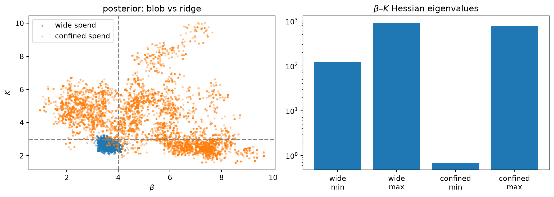
WE3 — The ridge made numerical (confined spend)
Setup.
Same model, same true parameters — \beta = 4, K = 3, n = 2, \lambda = 0.5 — but spend is now confined near x_0 = 3 with only small week-to-week variation. By WE1’s arithmetic, all operating points land near the same location on the Hill curve; all gradient vectors \nabla_\theta\mu_t point in nearly the same direction; the Fisher information matrix is nearly rank-one. Proof P1 predicts near-non-identifiability in the (\beta, K) direction, and Proof P2 predicts that the posterior along the resulting ridge will be proportional to the prior.
The MAP fit still passes.
MAP estimation converges; the fitted mean trajectory follows the observed sales series; residuals are small; posterior predictive checks pass. Nothing in the fit diagnostics signals trouble. This is the wound’s most insidious feature: good fit does not imply good recovery, and standard fit diagnostics cannot distinguish them.
The recovery has failed.
MAP estimation places K \approx 4.9 against the true K = 3 — a discrepancy of nearly two units. The model has found a different point on the (\beta, K) ridge that fits the confined-spend data equally well, consistent with the Proof P4 ridge \{(\beta, K) : \beta\cdot 9/(K^2+9) = \text{const}\}.
The ill-conditioning is visible in the Hessian.
Evaluate the Hessian of the negative log-posterior at the MAP. Its smallest eigenvalue quantifies the curvature in the flattest direction.
| Wide spend |
\approx 123 |
| Confined spend |
\approx 0.69 |
The ratio is roughly 180: the confined-spend posterior is about 180 times less curved in its flattest direction than the wide-spend posterior. The eigenvector associated with the tiny eigenvalue points along the (\beta, K) ridge — the direction Proof P1 identified as the null space of the nearly-singular Fisher information.
The Metropolis posterior confirms the width.
Run a Metropolis chain from the MAP under each design and examine the marginal posterior for K.
| Wide spend |
\approx 0.18 |
| Confined spend |
\approx 1.6 |
The confined-spend posterior for K has a standard deviation roughly nine times larger, and its mean sits far from the true K = 3. The chain is exploring a flat ridge, not a tight bowl.
Connecting to the proofs.
The anatomy is fully legible. By Proof P1, confined spend produces nearly collinear gradient vectors and a nearly singular I(\theta_0): the likelihood is nearly flat along the (\beta, K) ridge. By Proof P2, on a likelihood-flat ridge the posterior is proportional to the prior: the marginal posterior for K inherits the prior’s spread, not the data’s information. The wide posterior for K is not a sampler failure, not correctable by running longer chains, and not a sign of insufficient data — it is the correct Bayesian account of what the confined-spend design cannot tell us. Good fit, unrecoverable shape. The wound, now quantified.