26  Testing & Reliability

Canonical anchors: property-based testing (Claessen & Hughes); metamorphic testing (Chen et al.).

26.1 Motivation

Parts I through VI built the models — the response curves, the hierarchical priors, the samplers, the budget optimizer. Part VII has been about making that machinery trustworthy as software: Chapter 23 grounded its computation in finite-precision arithmetic, Chapter 24 structured its modules into an acyclic architecture, and Chapter 25 made its data durable in an append-only log. One question remains, and it is the one a practitioner is asked the moment a model influences a real budget: how do we know any of it is correct?

The honest difficulty is specific to statistical and optimization code. To test ordinary code we write an example test — fix an input, assert the expected output, assert f(x) == y. But a sampler returns a cloud of draws, an optimizer returns an allocation that depends on a tolerance and a starting point, and the prior store returns a posterior assembled from a stream of experiments. None of these has a closed-form “right answer” sitting ready to compare against. This is the oracle problem: the thing that would certify the output as correct — the oracle — does not exist in closed form for most of the MMM stack.

The driving question of this chapter is therefore: you cannot assert the sampler returns the “right” posterior, because there is no oracle — so how do you test statistical code, and how many random cases does it take to trust it?

The answer runs through the whole book. Every theorem we proved is a statement that must hold for all valid inputs: the fold is permutation-invariant and idempotent (Chapter 25), the dependency graph is acyclic (Chapter 24), adding a calibration factor never increases the EVPI (Chapter 22), and \kappa(X^\top X) \approx \kappa(X)^2 (Chapter 23). Each of these is exactly the kind of relation a test can check without knowing the exact output — and a relation that has been proved is the strongest oracle there is, because a test of it can fail only when the implementation is wrong. The theorems are the test oracles. Property-based and metamorphic testing turn them into running checks, and a short probabilistic argument — the keystone of this chapter — says how many random cases it takes before a passing test is genuine evidence of correctness.

26.2 Theory & Proofs

26.2.1 Rung 1 — The oracle problem: example tests versus property tests

An example test fixes a single input and asserts a single expected output, the familiar assert f(x) == y. It is the workhorse of ordinary software testing, and it has two limits worth naming precisely. First, it certifies the function only at the points enumerated: pass a hundred example tests and you have verified a hundred points of an infinite input space. Second, and more fundamental here, it presupposes a test oracle — a known correct output y to compare against.

For much of the MMM stack no such oracle exists. A sampler returns draws whose individual values are random; an optimizer returns an allocation that depends on tolerances and the starting point; the prior store returns a posterior assembled from a stream of calibration experiments. There is no closed-form y to write on the right-hand side of the assertion. This is the oracle problem, and it is the reason example testing alone cannot certify statistical or optimization code.

A property test sidesteps the missing oracle (Claessen and Hughes 2000). Instead of asserting that the output equals a specific value, it asserts a relation that must hold for all inputs — a universally quantified statement, checked not at one point but on many, typically randomly generated, cases. The shift is from a question about a value to a question about an invariant: not “is the output equal to this number?” but “does the output satisfy this property?” The property need not mention the exact output at all, which is exactly what lets it test code with no oracle.

26.2.2 Rung 2 — Metamorphic testing: the theorems are the oracles

A metamorphic relation is a relation between the outputs of a program on related inputs that must hold even when neither output’s exact value is known. The canonical example is permutation invariance: reordering the input must not change the result. We cannot say what sort does to one specific list without recomputing it, but we can say that sum(xs) == sum(shuffle(xs)) must hold for every list — and a violation is an unambiguous bug. Metamorphic testing checks such relations, and it is the natural fit for code with no oracle, because it tests the output’s behavior under transformation rather than the output’s value.

The observation that organizes this chapter is that the book’s proved theorems are exactly such relations — and therefore the strongest possible oracles. Each theorem is a relation that holds for all valid inputs by mathematical necessity, so a test of it can fail only when the implementation violates the theorem. The MMM stack supplies a ready stock of them:

  • Chapter 25 — permutation invariance: fold(log) == fold(permute(log)); the order in which calibration events arrive must not change the posterior.
  • Chapter 25 — idempotency under dedup: fold(log + duplicate) == fold(log); redelivering an already-folded event must leave the posterior unchanged.
  • Chapter 24 — acyclicity: a topological sort places every module if and only if the dependency graph is acyclic.
  • Chapter 22 — EVPI monotonicity: adding a ridge-aimed calibration factor never increases the expected value of perfect information.
  • Chapter 23 — conditioning: \kappa(X^\top X) \approx \kappa(X)^2 for the normal-equations Gram matrix.

The principle is then simple (Chen et al. 1998). A proved theorem asserts a relation that must hold; a property test is the empirical sampling of that theorem over the input space. Because the relation is a theorem, a failing test is never a false alarm about an expected value chosen wrongly — it is always a real defect in the code. The remaining question is quantitative: how many random samples does it take before a passing test is convincing evidence that no such defect exists?

26.2.3 Rung 3 — The probabilistic power of randomized testing

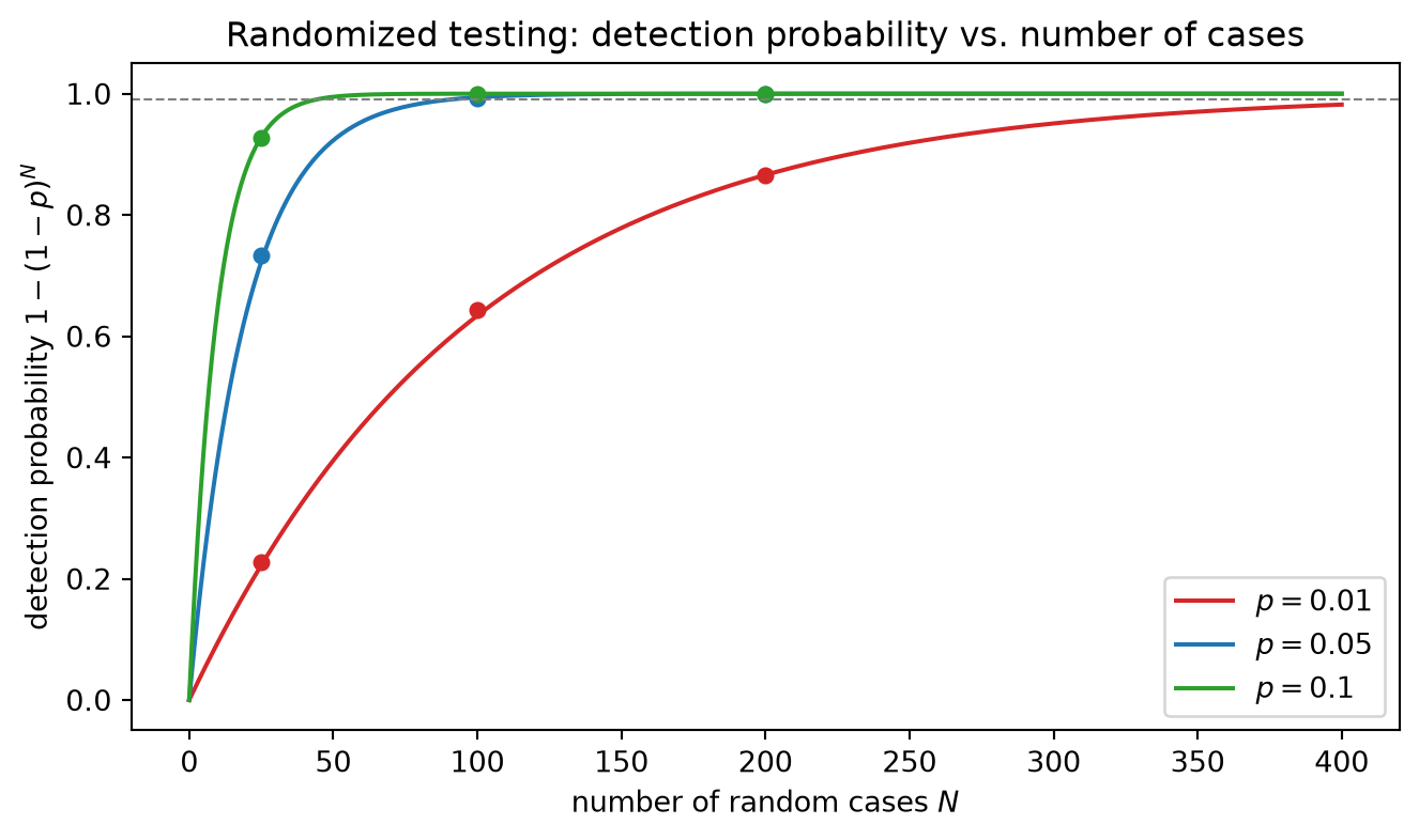
Random property testing turns “how much testing is enough?” into a probability question with a clean answer. Suppose a defect causes some property to fail on a fraction p \in (0, 1] of the input space — the failing fraction — and we draw N test cases independently and uniformly at random. How likely are we to catch it?

Theorem (detection probability). Under independent uniform sampling, the probability that at least one of N cases exposes the defect is

P_{\text{detect}}(N) = 1 - (1-p)^N \;\ge\; 1 - e^{-pN}.

Proof. A single random case lands in the failing region with probability p and misses it with probability 1 - p.

By independence, all N cases miss the failing region simultaneously with probability

(1-p)^N,

so at least one case hits it — exposing the defect — with the complementary probability 1 - (1-p)^N.

The exponential bound follows from the elementary inequality 1 - p \le e^{-p}, valid for every real p. Raising both sides to the Nth power gives (1-p)^N \le e^{-pN}, and therefore

P_{\text{detect}}(N) = 1 - (1-p)^N \;\ge\; 1 - e^{-pN}. \qquad \blacksquare

Corollary (sample size). To detect the defect with confidence at least 1 - \delta it suffices to drive the miss probability below \delta, i.e. (1-p)^N \le \delta. Taking logarithms and using \ln(1-p) \le -p,

N \;\ge\; \frac{\ln(1/\delta)}{p}.

The reading is the whole point of the keystone. A rarer bug — smaller failing fraction p — needs proportionally more cases, scaling as 1/p, and the desired confidence enters only logarithmically, so demanding ten times more certainty costs only a constant additive factor of cases. Concretely, a defect on a fraction p = 0.05 of inputs is caught by N = 100 random cases with probability 1 - 0.95^{100} \approx 0.994; a rarer defect with p = 0.01 needs N \ge \ln(100)/0.01 \approx 461 cases for 99\% confidence. (The bound is deliberately conservative — the exact requirement 0.99^{N} \le 0.01 is met at N = 459 — which is the safe direction for a test budget.) This is the guarantee an example test cannot offer: a random property test converts a target confidence directly into a number of cases.

26.2.4 Rung 4 — Numerical reliability: tolerances, seeds, and flakiness

Three hazards are specific to testing numerical and stochastic code, and each has a quantitative fix grounded in earlier chapters.

Tolerances. Finite precision (Chapter 23) makes exact-equality assertions on floating-point results simply wrong: two mathematically equal quantities computed by different routes rarely share every bit. The remedy is to compare within a tolerance,

|a - b| \;\le\; \texttt{atol} + \texttt{rtol}\,|b|,

and to size that tolerance to the conditioning of the computation — a result computed with condition number \kappa in unit roundoff u is accurate only to about \kappa u, so a tolerance set tighter than \kappa u asserts more precision than the arithmetic can deliver and will fail on correct code.

Reproducibility. A stochastic test must fix its random-number-generator seed. A seeded failure is replayable: the offending input can be regenerated, inspected, and minimized to a small counterexample. An unseeded property test that fails once and then passes on rerun has destroyed the very evidence needed to debug it — the failing case is gone. Seeding costs nothing and is non-negotiable for stochastic tests.

Flakiness. A Monte-Carlo estimate of a quantity — for instance the Chapter 22 EVPI — has standard error of order

\frac{\sigma}{\sqrt{n}},

for n draws. A regression test that asserts the estimate lies within a tolerance \texttt{tol} of a target will then pass or fail at random whenever \texttt{tol} \lesssim 3\sigma/\sqrt{n}, because the estimator’s own sampling noise exceeds the tolerance. The test is flaky — but not because the code is wrong; n and \texttt{tol} were sized inconsistently (Chapter 3). The fix is to make them consistent: raise n to shrink the standard error, or loosen \texttt{tol} to the estimator’s noise. Fixing the seed makes any single run deterministic, but the principled cure is to size the sample and the tolerance to each other.

26.2.5 Rung 5 — Reliability of the running system, and synthesis

Reliability is correctness under partial failure — retries, crashes, out-of-order and duplicate delivery — and the prior store of Chapter 25 already carries the two properties that provide it. Its operations are idempotent: deduplication by event_id makes a redelivered event a no-op, so an at-least-once retry cannot double-count. And it is replayable: because the posterior is a fold over an immutable, append-only log, a crash loses no committed state — the posterior rebuilds exactly by replaying the log. Together these mean failure does not corrupt the store, and — crucially for this chapter — both are testable as metamorphic relations, which is exactly how Worked Example 1 catches a store that lacks them.

Property and metamorphic tests take their place in a layered testing landscape: many fast example and unit tests pinning specific behaviors, a middle layer of property and metamorphic tests guarding the invariants the theorems guarantee, and a few slow end-to-end tests exercising the whole pipeline. The middle layer is what this chapter adds, and it is where the book’s mathematics pays a second dividend.

That dividend is the synthesis. The relations proved across the book now serve double duty — as specifications, stating what the system must compute, and as tests, checking that the implementation honors them on randomly generated inputs. Part VII therefore closes with the MMM system not merely built correctly in finite precision (Chapter 23), structured into a sound architecture (Chapter 24), and stored durably (Chapter 25), but verified to honor its own theorems. Chapter 27 takes the whole calibration–optimization system and exercises it end to end.

26.3 Worked Examples

26.3.1 WE1 — A metamorphic test catches what an example test misses

Consider two implementations of the prior-store fold: a correct one that deduplicates by event_id, and a buggy one that does not. The posterior precision is the prior precision 4 plus the contributions of the distinct calibration events — a lift experiment with s = 0.20 contributing 1/0.04 = 25, and one with s = 0.25 contributing 1/0.0625 = 16.

An example test folds a fixed log of the two distinct events and asserts the posterior precision equals

4 + 25 + 16 = 45.

This test passes for both implementations — the bug never manifests, because the fixed log contains no duplicate. The example test is blind to the defect.

Now the metamorphic idempotency test of Chapter 25: fold the log, then fold the same log with one event redelivered, and assert the two posteriors are equal. For the correct store the redelivered event is deduplicated and the posterior is unchanged at 45. For the buggy store the redelivered e_1 is counted twice,

4 + 25 + 25 + 16 = 70 \;\ne\; 45,

and the test fails. The theorem, used as an oracle, detects a defect the example test cannot see — and it does so without ever needing to know that 45 is the “right” answer.

26.3.2 WE2 — How many random cases? the detection probability in numbers

The dedup bug surfaces only when a generated log happens to contain a duplicate — say a fraction p = 0.05 of randomly generated logs, reflecting how often an at-least-once stream redelivers an event. A single example test built from distinct events sits forever in the 95\% of inputs that miss the defect and never catches it. A campaign of N = 100 random property checks, by contrast, catches it with probability

1 - 0.95^{100} \approx 0.994.

For a rarer defect with failing fraction p = 0.01, reaching 99\% confidence (\delta = 0.01) requires

N \;\ge\; \frac{\ln(100)}{0.01} \approx 461

random cases. The sample-size rule converts a desired confidence directly into a test budget: pick the bug rarity you want to guard against and the confidence you need, and read off the number of cases.

26.3.3 WE3 — A flaky Monte-Carlo test, and how to size it

Suppose the Chapter 22 EVPI is estimated by Monte Carlo with n draws, so the estimate carries a standard error of about \sigma/\sqrt{n}. A regression test that asserts the estimate is within a tolerance \texttt{tol} of a target EVPI will pass or fail at random — it is flaky — whenever

\texttt{tol} \;<\; \frac{3\sigma}{\sqrt{n}},

because the estimator’s own noise exceeds the tolerance. With \sigma \approx 0.5 and n = 10^4 the standard error is 0.005, so a tolerance of 0.002 flakes — it is tighter than the noise — while 0.02 is safe. The alternative is to shrink the noise: raising n tightens \sigma/\sqrt{n} until the desired tolerance becomes safe. Fixing the seed makes one run deterministic, but the principled fix is to size n and \texttt{tol} to each other.

26.4 Code Tie-in

import numpy as np
import matplotlib.pyplot as plt

# === The prior store as a fold (Chapter 25), correct vs. buggy ============
# Posterior precision = prior + sum of DISTINCT calibration contributions.
PRIOR = 4.0
BASE_LOG = [
    {"event_id": "e1", "prec": 25.0},   # lift, s = 0.20 -> 1/0.04 = 25
    {"event_id": "e2", "prec": 16.0},   # lift, s = 0.25 -> 1/0.0625 = 16
]

def fold(events, prior=PRIOR, dedup=True):
    """Correct store dedups by event_id; the buggy store (dedup=False) does not."""
    seen, prec = set(), prior
    for ev in events:
        if dedup and ev["event_id"] in seen:
            continue
        seen.add(ev["event_id"])
        prec += ev["prec"]
    return prec

correct = lambda log: fold(log, dedup=True)
buggy   = lambda log: fold(log, dedup=False)

def distinct(log):
    """The distinct-by-event_id events, preserving first-seen order."""
    seen, out = set(), []
    for ev in log:
        if ev["event_id"] not in seen:
            seen.add(ev["event_id"]); out.append(ev)
    return out

# === A property-test harness (no third-party testing library) =============
def make_log(rng, p):
    """A log of distinct events; with probability p, append a duplicate (a retry)."""
    log = [dict(ev) for ev in BASE_LOG]
    if rng.random() < p:
        log.append(dict(log[rng.integers(len(log))]))   # duplicate one event
    return log

def mr_idempotent(fold_fn, log):
    """Metamorphic relation (Ch.25): re-folding a duplicated event must not change the result."""
    dup = log + [dict(log[0])]
    return fold_fn(dup) == fold_fn(log)

def mr_dup_invariant(fold_fn, log):
    """Metamorphic relation (Ch.25): the result must be invariant to duplicate delivery.
    Violated by the buggy store exactly when `log` already contains a duplicate."""
    return fold_fn(log) == fold_fn(distinct(log))

# === 1. Example test vs. metamorphic test (WE1) ===========================
example_log = [dict(ev) for ev in BASE_LOG]      # fixed, distinct -> precision 45
print("1) example test (fixed distinct log -> precision 45)")
print(f"   correct fold = {correct(example_log)}   buggy fold = {buggy(example_log)}")
assert correct(example_log) == 45.0
assert buggy(example_log)   == 45.0              # example test PASSES for both

dup_log = example_log + [dict(example_log[0])]   # e1 retried
print("   idempotency metamorphic test (fold(log+dup) == fold(log)):")
print(f"   correct: {correct(dup_log)} vs {correct(example_log)}   "
      f"buggy: {buggy(dup_log)} vs {buggy(example_log)}")
assert mr_idempotent(correct, example_log) is True     # holds for the correct store
assert mr_idempotent(buggy,   example_log) is False    # FAILS for the buggy store (70 != 45)
assert buggy(dup_log) == 70.0

# === 2. Detection probability of randomized testing (WE2 / keystone) ======
# A randomly generated log contains a natural duplicate with probability p, and the
# buggy store violates duplicate-invariance only on those logs -> per-case detection = p.
def P_detect(p, N):
    return 1.0 - (1.0 - p) ** N

rng = np.random.default_rng(26)
p, N = 0.05, 100

per_case = sum(not mr_dup_invariant(buggy, make_log(rng, p)) for _ in range(N))
print("\n2) detection probability (keystone)")
print(f"   single random cases that caught the bug: {per_case}/{N}  (expected ~{p*N:.0f})")
print(f"   P_detect(p=0.05, N=100) = {P_detect(0.05, 100):.4f}")

# Empirical campaign detection rate: does a campaign of N cases catch the bug at least once?
campaigns = 4000
hits = 0
for _ in range(campaigns):
    found = any(not mr_dup_invariant(buggy, make_log(rng, p)) for _ in range(N))
    hits += found
emp_rate = hits / campaigns
print(f"   empirical detection rate over {campaigns} campaigns of N=100 = {emp_rate:.4f}")
assert abs(emp_rate - P_detect(p, N)) < 0.02      # tolerance sized to sampling noise (Rung 4)

# sample size for a rarer defect
delta = 0.01
N_needed = int(np.ceil(np.log(1/delta) / 0.01))   # conservative bound
print(f"   p=0.01, delta=0.01 -> N >= ln(1/delta)/p = {N_needed}")
assert N_needed == 461

# === Figure: detection-probability curves with empirical points overlaid ===
Ns = np.arange(0, 401)
fig, ax = plt.subplots(figsize=(7, 4.2))
for pp, color in zip([0.01, 0.05, 0.10], ["tab:red", "tab:blue", "tab:green"]):
    ax.plot(Ns, P_detect(pp, Ns), color=color, label=f"$p={pp}$")
    for Npt in [25, 100, 200]:                      # empirical points
        h = sum(any(not mr_dup_invariant(buggy, make_log(rng, pp)) for _ in range(Npt))
                for _ in range(800))
        ax.plot(Npt, h/800, "o", color=color, markersize=5)
ax.axhline(0.99, ls="--", lw=0.8, color="gray")
ax.set_xlabel("number of random cases $N$")
ax.set_ylabel("detection probability $1-(1-p)^N$")
ax.set_title("Randomized testing: detection probability vs. number of cases")
ax.legend()
plt.tight_layout()
plt.show()
print("\nAll assertions passed.")
1) example test (fixed distinct log -> precision 45)
   correct fold = 45.0   buggy fold = 45.0
   idempotency metamorphic test (fold(log+dup) == fold(log)):
   correct: 45.0 vs 45.0   buggy: 70.0 vs 45.0

2) detection probability (keystone)
   single random cases that caught the bug: 2/100  (expected ~5)
   P_detect(p=0.05, N=100) = 0.9941
   empirical detection rate over 4000 campaigns of N=100 = 0.9962
   p=0.01, delta=0.01 -> N >= ln(1/delta)/p = 461


All assertions passed.

26.5 Exercises

26.5.1 C – Conceptual / Reading Comprehension

  1. State the oracle problem in your own words, and explain why it makes a sampler or a budget optimizer hard to test with example tests. What does a property test assert instead of an expected value?
  2. Why is a proved theorem the strongest possible test oracle? In particular, when a property test of a theorem fails, what can and cannot be the cause?
  3. Why does an unseeded stochastic test that fails once resist debugging? What single practice fixes this, and what does it cost?
  4. Give the metamorphic relation, drawn from an earlier chapter, that you would use to test each of: the prior-store fold, the module dependency graph, and the normal-equations solver.

26.5.2 B – By Hand

  1. A defect fails on a fraction p = 0.02 of inputs. Compute the detection probability for N = 50 and for N = 200 random cases.
  2. Using the sample-size rule N \ge \ln(1/\delta)/p, how many random cases are needed to detect a defect with failing fraction p = 0.005 at confidence 1 - \delta = 0.99?
  3. A Monte-Carlo test estimates a quantity with population standard deviation \sigma = 0.8 using n = 2500 draws. Compute the standard error, and give a tolerance that is not flaky (use the 3\sigma/\sqrt{n} threshold). If you must assert to within \texttt{tol} = 0.01, what is the smallest n that keeps the test non-flaky?

26.5.3 P – Prove It

  1. Prove that N independent, uniformly drawn random cases detect a defect of failing fraction p with probability 1 - (1-p)^N, and derive the sample-size rule N \ge \ln(1/\delta)/p for confidence 1 - \delta. State precisely where independence is used and which inequality gives the bound.
  2. Show that a metamorphic relation guaranteed by a proved theorem is a sound oracle: a test of it raises a failure only when the implementation violates the theorem, never as a false alarm. (Argue from the universal quantification: the theorem holds for all valid inputs, so any observed violation witnesses an implementation that does not compute the specified function.)

26.5.4 A – Applied / Code

  1. Extend the Code Tie-in with a third metamorphic relation drawn from another chapter — for example Chapter 24 acyclicity (build a small dependency graph, assert a topological order exists) or Chapter 22 EVPI monotonicity (assert that adding a calibration factor does not increase the EVPI). Inject a defect that violates your relation (a back-edge in the graph; a factor that worsens the EVPI), and confirm the metamorphic test catches it while a plausible example test does not.
  2. Estimate the empirical detection rate of your new test as a function of N and overlay it on the keystone curve 1 - (1-p)^N; report the failing fraction p you observe.
  3. Take any Monte-Carlo assertion in the cell, tighten its tolerance until the test becomes flaky across seeds, then restore reliability by sizing n up to the tolerance (rather than loosening the tolerance). Report the n at which the test becomes reliable again.

26.6 Summary

Key concepts

  • The oracle problem: samplers, optimizers, and the prior store have no closed-form expected output, so example tests (assert f(x) == y) cannot certify them.
  • A property test asserts an invariant that holds for all inputs, checked on many random cases, rather than a single expected value.
  • A metamorphic relation relates outputs on related inputs (e.g. permutation invariance) and needs no oracle; the book’s proved theorems are exactly such relations, hence the strongest oracles.
  • Numerical reliability has three hazards — exact-equality assertions (use tolerances \approx \kappa u), unseeded stochastic tests (fix the seed for replayability), and flaky Monte-Carlo tests (size n and \texttt{tol} to each other).
  • Reliability is correctness under partial failure; idempotency and replayability (Chapter 25) provide it, and both are testable as metamorphic relations.
  • The relations proved across the book serve double duty as specifications and as tests — Part VII ends with the system not just built but verified.

Key identities

  • example test certifies enumerated points; a property test certifies an invariant over all inputs
  • metamorphic relations as oracles: \texttt{fold(log)} = \texttt{fold(permute(log))} and \texttt{fold(log + dup)} = \texttt{fold(log)}
  • detection probability P_{\text{detect}} = 1 - (1-p)^N \ge 1 - e^{-pN}
  • sample-size rule N \ge \ln(1/\delta)/p for confidence 1 - \delta
  • Monte-Carlo flakiness threshold \texttt{tol} \gtrsim 3\sigma/\sqrt{n}
  • idempotent + replayable \Rightarrow reliable under retry

The oracles of this chapter are the theorems of Chapters 22–25, and the keystone says how many random cases turn them into trust. Chapter 27 assembles the whole calibration–optimization system and exercises it end to end.

Chen, T. Y., S. C. Cheung, and S. M. Yiu. 1998. Metamorphic Testing: A New Approach for Generating Next Test Cases. HKUST-CS98-01. Department of Computer Science, Hong Kong University of Science; Technology.
Claessen, Koen, and John Hughes. 2000. QuickCheck: A Lightweight Tool for Random Testing of Haskell Programs.” Proceedings of the Fifth ACM SIGPLAN International Conference on Functional Programming (ICFP), 268–79.