Motivation
Every model in Parts I through VI ran on a substrate this book has so far taken for granted. The normal equations of Chapter 4, the Gaussian posteriors of Chapters 5 and 6, the per-sample work of the samplers in Chapters 8 through 10, the optimizers of Chapters 12 through 14, and the Kalman and prior-store recursions of Chapters 17 and 22 were all written in exact arithmetic on paper and then executed in finite-precision arithmetic at finite cost. This chapter opens Part VII by making that substrate precise. The driving question is the one a practitioner eventually meets the hard way: your model fit, sampler, and optimizer all run on finite-precision arithmetic at finite cost — when does that silently corrupt the answer, and what does it cost to scale?
The chapter has two pillars. The first, and its center of gravity, is floating-point arithmetic and conditioning: the question of when finite precision quietly destroys an answer that the mathematics says is well-defined. The second, supporting, pillar is algorithmic cost: the asymptotic price of the linear-algebra and sampling primitives the MMM stack runs, and how that price scales with the number of channels and the number of draws. The two are not separate concerns. A computation can be cheap and wrong, or correct and unaffordable; an engineer needs to see both axes at once.
The payoff that unifies the chapter is a single observation: the Chapter 16 identifiability ridge is also a numerical conditioning problem. When two spend channels move nearly together in the historical data, the design matrix has two nearly parallel columns, its smallest singular value is nearly zero, and its condition number is enormous. The statistical statement — the data cannot identify the contrast between those channels — and the numerical statement — a naive solve loses most of its digits along that contrast — are the same fact seen from two sides. The very direction that the calibration factor of Chapter 21 was built to compress is the direction in which floating-point arithmetic silently fails.
Throughout, the discussion stays anchored to the computational stack the book has already built — the regression solve, the Gaussian posterior, the samplers, the ridge — rather than surveying computer science for its own sake. Sorting and data structures appear only as passing context; the working material is the arithmetic and the cost of the operations an MMM actually performs.
Theory & Proofs
The five rungs build from cost to correctness. Rung 1 fixes the cost model and prices the linear-algebra primitives the MMM stack runs. Rung 2 states the floating-point model and the basic rounding bound. Rung 3 isolates catastrophic cancellation, the most common way a correct formula returns a wrong number. Rung 4 is the keystone: the condition number, and the proof that forming the normal equations squares it — the result that ties the Chapter 16 ridge to numerical loss of precision. Rung 5 closes on backward stability and the practical rules the rest of the stack depends on.
Rung 1 — The cost model and asymptotic complexity
To reason about cost we count elementary operations — arithmetic, comparisons, memory accesses — as a function of the input size n, ignoring constant factors and lower-order terms. This is the RAM model, and the bookkeeping is the asymptotic notation O(\cdot) for upper bounds, \Omega(\cdot) for lower bounds, and \Theta(\cdot) for tight bounds. The point is not the exact instruction count, which depends on the machine, but how the count grows: an O(n^2) routine and an O(n^3) routine differ by a factor that widens without bound as the problem scales.
The primitives the MMM stack runs have well-known costs. A matrix–vector product is O(n^2); a matrix–matrix product is O(n^3); solving a triangular system by back-substitution is O(n^2). The workhorse for a symmetric positive-definite system — and every Gaussian posterior precision is one — is the Cholesky factorization A = LL^\top, whose cost sets the price of a posterior solve.
Proposition (Cholesky flop count). Factorizing an n \times n symmetric positive-definite matrix by Cholesky costs \approx n^3/3 multiply–add operations.
Proof. The factorization computes the columns of L in turn. Producing the k-th column requires forming an inner product of length about k for each of the roughly n - k entries below the diagonal, plus the diagonal entry itself — on the order of k(n-k) multiply–adds, dominated near the diagonal by a cost that sums to the same order as \sum_k k^2.
Summing the dominant term over all columns gives the closed form:
\sum_{k=1}^{n} k^2 = \frac{n(n+1)(2n+1)}{6} \approx \frac{n^3}{3}.
The total is therefore \Theta(n^3) with leading constant 1/3. \blacksquare
The reading for an MMM is immediate. A model with d channels has a d \times d posterior precision, so a single posterior solve costs \Theta(d^3); drawing S posterior samples that each require a solve multiplies that by S. Doubling the number of channels octuples the per-solve cost. This is why the dimension of the model is a first-order engineering constraint, not a detail — a theme Rung 4 sharpens from cost into correctness. (Sorting, searching, and the classical data structures of CLRS are the broader context of this rung, but the MMM stack leans almost entirely on dense linear algebra, so that is where we stay.)
Rung 2 — The IEEE-754 model and the rounding bound
A double-precision number is stored as \pm\, m \cdot 2^{e} with a 52-bit fractional mantissa m. Only finitely many such numbers exist, so most real numbers must be rounded to the nearest representable one. The granularity of that rounding is captured by two constants: machine epsilon \varepsilon_{\text{mach}} = 2^{-52} \approx 2.22 \times 10^{-16}, the gap between 1 and the next larger representable number, and the unit roundoff u = 2^{-53} \approx 1.11 \times 10^{-16}, half that gap, which bounds the relative error of rounding a single value.
Theorem (floating-point axiom). For any two representable numbers x, y and any basic operation \mathbin{op} \in \{+, -, \times, \div\}, the computed result satisfies
\mathrm{fl}(x \mathbin{op} y) = (x \mathbin{op} y)(1 + \delta), \qquad |\delta| \le u.
Proof. Let z = x \mathbin{op} y be the exact result, and suppose z lies between consecutive representable numbers separated by a spacing \Delta at that magnitude. Round-to-nearest returns the closer of the two, so the absolute error is at most half the spacing:
|\mathrm{fl}(z) - z| \le \tfrac{1}{2}\Delta.
At magnitude |z| the spacing relative to the value is \Delta / |z| \le 2u, so the relative error is bounded by
\frac{|\mathrm{fl}(z) - z|}{|z|} \le \frac{\Delta}{2|z|} \le u.
Writing \delta = (\mathrm{fl}(z) - z)/z gives \mathrm{fl}(z) = z(1+\delta) with |\delta| \le u. \blacksquare
A single operation is therefore accurate to a relative error of about 10^{-16} — sixteen good digits. The danger is never one operation; it is that these errors compose, and that certain combinations amplify them catastrophically. Rung 3 is the canonical amplifier.
Rung 3 — Catastrophic cancellation
The rounding bound says each operand is known to a small relative error. Subtraction of two nearly-equal numbers converts that small relative error into a large one, because the result is small while the absolute errors carried by the operands are not.
Suppose the operands themselves carry rounding error, \hat x = x(1 + \delta_x) and \hat y = y(1 + \delta_y) with |\delta_x|, |\delta_y| \le u. The error in their difference is \hat x - \hat y - (x - y) = x\delta_x - y\delta_y, whose magnitude is at most (|x| + |y|)\,u. Dividing by the true difference gives the relative error:
\frac{\bigl|(\hat x - \hat y) - (x - y)\bigr|}{|x - y|} \le \frac{|x| + |y|}{|x - y|}\,u.
The amplification factor (|x| + |y|)/|x - y| is harmless when x and y are far apart but diverges as x \to y: subtracting numbers that agree in their leading digits cancels those digits and promotes the trailing rounding noise to the leading position.
The textbook MMM trap is the one-pass variance. The algebraic identity \operatorname{Var}(x) = \overline{x^2} - \bar{x}^2 is exact on paper, but when the mean is large relative to the spread, \overline{x^2} and \bar{x}^2 are two large, nearly-equal numbers, and their difference cancels catastrophically. The two-pass form \overline{(x - \bar{x})^2} subtracts the mean first, while the operands are still full-precision, and never forms the dangerous difference of large quantities. Worked Example 1 shows the one-pass formula returning exactly zero where the two-pass form is exact.
Rung 4 — The condition number and \kappa(X^\top X) = \kappa(X)^2 (keystone)
Conditioning measures how much a problem amplifies input error, independent of the algorithm used to solve it. For a linear system the relevant quantity is the condition number of the matrix, defined in the 2-norm by
\kappa(A) = \lVert A \rVert \, \lVert A^{-1} \rVert = \frac{\sigma_{\max}(A)}{\sigma_{\min}(A)},
the ratio of largest to smallest singular value. The role it plays is captured by the forward-error bound: when Ax = b is solved with a relatively perturbed right-hand side or matrix, the relative error in the solution is bounded by \kappa(A) times the relative perturbation. Since rounding makes the perturbation about u, a solve loses roughly \log_{10}\kappa(A) decimal digits. Conditioning is a property of the problem; no algorithm can recover digits that the conditioning has already put out of reach.
The keystone concerns what happens when least squares is solved through the normal equations X^\top X\, \beta = X^\top y — the route Chapter 4 wrote down — rather than through a factorization of X directly.
Theorem. In the 2-norm, \kappa(X^\top X) = \kappa(X)^2.
Proof. Take the singular value decomposition X = U \Sigma V^\top, with U and V orthogonal and \Sigma diagonal carrying the singular values \sigma_i(X). Then
X^\top X = V \Sigma^\top U^\top U \Sigma V^\top = V \Sigma^2 V^\top,
using U^\top U = I. This is an eigendecomposition of X^\top X, so its singular values are the diagonal entries of \Sigma^2, namely \sigma_i(X)^2.
Taking the ratio of largest to smallest gives the result directly:
\kappa(X^\top X) = \frac{\sigma_{\max}(X)^2}{\sigma_{\min}(X)^2} = \left(\frac{\sigma_{\max}(X)}{\sigma_{\min}(X)}\right)^2 = \kappa(X)^2.
\blacksquare
Forming and solving the normal equations therefore squares the condition number and doubles the digits lost. A design that loses six digits when solved through a QR or SVD factorization of X — conditioning \kappa(X) — loses twelve when solved through X^\top X — conditioning \kappa(X)^2. The practical rule follows: solve least squares by factorizing X (QR or SVD), never by forming X^\top X.
Here the chapter’s two threads meet. The Chapter 16 identifiability ridge is precisely the case of near-collinear spend columns: two columns of X that are nearly parallel make \sigma_{\min}(X) \approx 0 and \kappa(X) enormous. The statistical statement that the data cannot identify the contrast between those channels is the numerical statement that X is nearly singular along that contrast — one fact, two languages. And the direction in which a naive normal-equations solve discards all its precision is exactly the contrast direction that the calibration factor of Chapter 21 was constructed to compress. Calibration heals the ridge statistically and conditions the problem numerically.
Rung 5 — Backward stability and the practical upshot
Conditioning bounds the best any algorithm can do; stability asks whether a given algorithm achieves it. An algorithm is backward stable if its computed output is the exact solution of a slightly perturbed input — the backward error is on the order of u. For such an algorithm the forward error is bounded by conditioning times backward error, about \kappa(A)\, u: you cannot beat the conditioning, but a backward-stable method does not make matters worse than the problem already is.
The classical factorizations are backward stable. Solving a symmetric positive-definite system by Cholesky, and solving least squares by QR, both achieve accuracy on the order of \kappa\, u (Trefethen and Bau 1997). This is what licenses the practical rules the rest of the stack silently depends on: never invert a matrix when you can solve a system; never form X^\top X when you can factorize X; sum many terms with a compensated or pairwise scheme rather than naively; compute a variance in two passes, not one. None of these change what the mathematics says; they protect what the arithmetic delivers.
These rules also set the agenda for the rest of Part VII. The cost bounds of Rung 1 and the numerical hazards of Rungs 2 through 4 are properties of single computations; an MMM in production runs them repeatedly, on growing data, behind interfaces other systems depend on. Chapter 24 (software architecture), Chapter 25 (data engineering), and Chapter 26 (testing and reliability) are the engineering that preserves cost and correctness at that scale.
Worked Examples
Three worked examples make the rungs concrete: the first shows a correct formula returning a wrong answer, the second shows the keystone squaring on the ridge, and the third prices the Gaussian solve.
WE1 — Catastrophic cancellation in the variance
Take three data points clustered far from the origin, x = 10^8 + \{1, 2, 3\}, whose population variance is that of \{1, 2, 3\}, namely \tfrac{2}{3} \approx 0.667. Compute the variance two algebraically-identical ways.
The one-pass formula forms \overline{x^2} - \bar{x}^2. Both terms are about 10^{16}, and they agree to far more than sixteen digits before the small variance appears, so in double precision their difference rounds to exactly 0.0 — every significant digit of the answer has cancelled away. The two-pass formula \overline{(x - \bar{x})^2} subtracts the mean of 10^8 + 2 while the data are still full-precision, reducing the operands to \{-1, 0, 1\} before squaring, and returns 0.667 exactly.
The lesson is that algebraic equivalence is not numerical equivalence. The two formulas compute the same real number and disagree completely in floating-point, because one of them passes through the difference of two large, nearly-equal quantities and the other does not.
WE2 — \kappa(X^\top X) = \kappa(X)^2 and the digits lost (keystone)
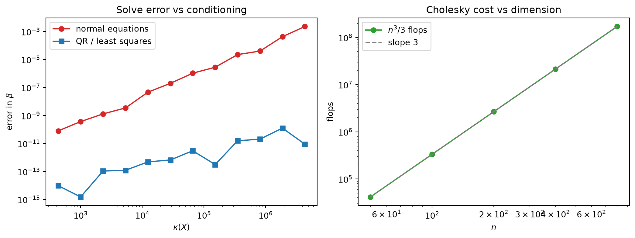
Construct a near-collinear design: a column t of 50 evenly spaced values and a second column equal to the first plus a perturbation of size 10^{-6}. The two columns are almost parallel — the Chapter 16 ridge in miniature. Numerically the design has condition number \kappa(X) \approx 4.3 \times 10^{6}, and the normal-equations matrix has
\kappa(X^\top X) \approx 1.9 \times 10^{13} = \kappa(X)^2,
the ratio \kappa(X^\top X)/\kappa(X)^2 equal to 1.002 — the squaring of Rung 4, observed (the conditioning here is moderate enough, \kappa(X)^2 \ll u^{-1}, that the ratio is itself computed cleanly).
The consequence is visible in a solve for a known coefficient \beta = (2, -1). Recovering \beta through the normal equations X^\top X\, \beta = X^\top b gives an error of about 8.1 \times 10^{-4}; recovering it through a QR/least-squares factorization of X gives an error of about 8.8 \times 10^{-11}. The two differ by a factor of roughly 10^{7} — on the order of the extra \kappa(X) that forming X^\top X introduced. The worse the identification, the more digits the naive route discards: the ridge as a numerical object.
WE3 — The O(n^3) cost of the Gaussian solve
The price of a posterior solve is the Cholesky cost of Rung 1, \approx n^3/3 flops. Tabulating the analytical flop count at growing dimension shows the cubic scaling cleanly: from n to 2n the count n^3/3 rises by a factor of 2^3 = 8, so each doubling of the channel count octuples the per-solve cost. At n = 200, 400, 800 the analytical counts are about 2.7 \times 10^{6}, 2.1 \times 10^{7}, and 1.7 \times 10^{8}, each 8\times the last.
Wall-clock timing follows the same cubic trend but only loosely at small sizes, because threaded linear-algebra libraries carry fixed overheads and parallelism that distort the constant; this is why the Code Tie-in asserts the exact analytical flop ratio rather than any measured time. The reading for an MMM is that dimension is expensive in a precise, cubic way: a model with twice the channels costs eight times as much per solve, and that cost is paid once per posterior draw when the model is sampled.
Exercises
C – Conceptual / Reading Comprehension
C1. A colleague solves the MMM least-squares problem by computing inv(X.T @ X) @ X.T @ y. Explain, using the condition number, why this is the worst of the available routes on two counts — forming X^\top X and then inverting it — and state what they should do instead.
C2. Define machine epsilon for double precision. Then explain why catastrophic cancellation is described as a loss of relative accuracy: what stays bounded, what shrinks, and why their ratio is what matters.
C3. In what precise sense is the Chapter 16 identifiability ridge simultaneously a statistical object and a numerical object? Identify the single matrix quantity that is large in both stories and explain why.
B – By Hand
B1. Double precision has a 52-bit mantissa. Compute the unit roundoff u, and state how many correct decimal digits a single floating-point operation delivers.
B2. A 2 \times 2 design has singular values \sigma_{\max} = 4 and \sigma_{\min} = 4 \times 10^{-4}. Compute \kappa(X) and \kappa(X^\top X), and state how many decimal digits a backward-stable solve loses through each of the two routes.
B3. For the data x = \{10^6 + 1,\ 10^6 + 2,\ 10^6 + 3\}, write out the one-pass quantity \overline{x^2} - \bar{x}^2 and the two-pass quantity \overline{(x - \bar{x})^2} symbolically, and explain which large intermediate quantities the one-pass route forms that the two-pass route never does.
P – Prove It
P1. Using the singular value decomposition X = U\Sigma V^\top, prove that \kappa(X^\top X) = \kappa(X)^2 in the 2-norm. State clearly where orthogonality of U and V is used.
P2. Prove the floating-point rounding bound: under round-to-nearest, \mathrm{fl}(x \mathbin{op} y) = (x \mathbin{op} y)(1 + \delta) with |\delta| \le u. Then, modelling each operand as carrying relative error at most u, derive the catastrophic-cancellation bound \frac{|x| + |y|}{|x - y|}\,u for the relative error of x - y.
A – Applied / Code
A1. Sweep the conditioning of X by shrinking the perturbation between its two columns, and plot the realized solve error of the normal-equations route and the QR route against \kappa(X) on log–log axes. Confirm the slopes: normal equations rising as \kappa^2 u, QR as \kappa u.
A2. Add a calibration-style rank-one increment to the precision (as in Chapter 21) aimed at the ill-conditioned contrast direction, and show that it raises the smallest singular value, lowers \kappa(X), and reduces the realized solve error together — the ridge healed numerically as well as statistically.