Motivation
Chapter 21 folded a single calibration estimate into the posterior and showed it heal the identifiability ridge: one experiment, aimed at the direction the observational data left flat, compressing the allocation posterior and shrinking the Chapter 18 EVPI gap. But a measurement program is never one experiment. An organization running an MMM accumulates geo-lift tests, holdout studies, and matched-market experiments over years — some recent and well-randomized, some stale, some of doubtful design, some measuring the same quantity and disagreeing. The driving question of this chapter is the one that follows directly: you will run not one experiment but many, over years, of varying quality and freshness. How do you accumulate them correctly — and does the decision actually converge?
The answer is the prior store: an append-only, versioned ledger of calibration likelihood factors, keyed by the secant / tangent / validation taxonomy of Chapters 20 and 21. Each experiment enters as a factor on a functional of the response-curve parameters; the store is the running product of those factors, maintained as evidence arrives. Four mechanisms make the accumulation correct and its payoff provable. Sequential updating equals batch updating, so studies can be appended one at a time without re-fitting. Power-prior discounting and temporal decay down-weight stale or low-credibility studies, so the store tracks a drifting landscape. Hierarchical pooling reconciles studies that conflict, so disagreement inflates uncertainty rather than being compounded into false confidence. And the keystone: as ridge-aimed studies accumulate, the EVPI gap decays monotonically to zero — the loop the book has been building provably converges.
The full software-engineering build of the store — storage, schema migrations, governance, the pipeline that re-optimizes whenever a study lands — is the subject of Part VII. This chapter is the mathematics of evidence accumulation: the capstone of Part VI, where the calibration–optimization loop is closed and shown to converge.
Throughout, the anchor response curve is again S(x;\theta) = \theta\sqrt{x} with true scale \theta = 2, and the ridge is the two-channel coefficient model (a_1, a_2) of Chapters 18 and 21: the attribution-contrast direction u = (1,-1)/\sqrt{2} is the near-flat eigendirection the observational data barely identify, and the direction every calibration study is aimed at.
Theory & Proofs
The five rungs build from mechanism to payoff. Rung 1 establishes the store as a product of likelihood factors and proves that updating it sequentially equals the batch posterior. Rung 2 adds power-prior discounting and temporal decay, the weights that keep the store current. Rung 3 handles conflict: how to pool studies that disagree beyond their stated noise. Rung 4 is the keystone — the proof that the EVPI gap decays monotonically to zero as the store fills with ridge-aimed evidence. Rung 5 reads the mathematics back as a data-product schema and hands the engineering build to Part VII.
Rung 1 — The store as a product of likelihood factors (sequential = batch). The prior store is, mathematically, the running product of calibration factors. Begin with the observational posterior p_0(\theta) \propto p(\theta)\,L_{\text{obs}}(\theta \mid D) and let experiments arrive as a stream \hat g_1, \dots, \hat g_k, each contributing a calibration factor L_j(\hat g_j \mid \theta). The store maintains the posterior by the Bayesian recursion p_j(\theta) \propto p_{j-1}(\theta)\,L_j(\hat g_j \mid \theta): each new study multiplies the current posterior by its factor.
Theorem (cumulative meta-analysis / sequential = batch). Unrolling the recursion,
p_k(\theta) \;\propto\; p_0(\theta) \prod_{j=1}^{k} L_j(\hat g_j \mid \theta) ,
so folding studies in one at a time — sequentially, as the store receives them — yields exactly the batch posterior that conditions on all k experiments at once.
Proof. By induction on k. For the base case k = 1, the recursion gives p_1 \propto p_0 L_1, which is the product form. For the inductive step, assume p_{k-1} \propto p_0 \prod_{j=1}^{k-1} L_j. The recursion then gives
\begin{aligned}
p_k &\propto p_{k-1} L_k && \text{(recursion)} \\
&\propto p_0 \prod_{j=1}^{k-1} L_j \cdot L_k && \text{(inductive hypothesis)} \\
&= p_0 \prod_{j=1}^{k} L_j && \text{(associativity).}
\end{aligned}
That the joint experimental likelihood factors as \prod_j L_j is licensed by conditional independence of the experiments given \theta: each randomization is a separate data source, so conditioning on the parameters renders the experimental outcomes independent. \blacksquare
This is the correctness guarantee of an incremental store. Because multiplication commutes and associates, the order in which studies are appended does not change the posterior, and a study can be folded in without re-fitting the model from scratch. The MMM reading is operational: the store is an append-only ledger of likelihood factors, and the live posterior is their product, recomputable at any time by replaying the ledger.
Rung 2 — Power-prior discounting and temporal decay. Not every study deserves full weight. A stale study run under a media landscape that no longer holds, or a geo experiment with a suspect randomization, should enter the store down-weighted. The power prior formalizes this by raising each calibration factor to a fractional power L_j^{w_j} with w_j \in [0,1], so the accumulated posterior is
p_k(\theta) \;\propto\; p_0(\theta) \prod_{j=1}^{k} L_j(\hat g_j \mid \theta)^{w_j} .
The weight is composed as w_j = (\text{design credibility}) \times \rho^{\,t_{\text{now}} - t_j}, where the temporal decay factor \rho^{\,t_{\text{now}} - t_j} discounts a study that is t_{\text{now}} - t_j time units old at decay rate \rho < 1. A recent, well-designed study has w near 1 (the standard update); a stale or methodologically weak study has w near 0; a validation-tier study sets w = 0 and never enters the likelihood at all. There is a subtlety, due to Ibrahim & Chen (Ibrahim and Chen 2000): raising a likelihood to a power changes its normalizing constant, and when w is itself treated as an unknown to be inferred, that constant must be carried or the posterior over w is distorted. With w fixed by the store’s design policy — the case here — the factor is a clean tempered likelihood and no normalization issue arises. The effect of temporal decay is that the store forgets: old evidence is continuously down-weighted, so the live posterior tracks a drifting landscape rather than anchoring forever to the first study run.
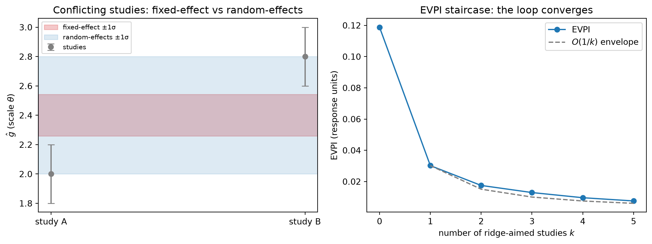
Rung 3 — Hierarchical pooling of conflicting studies. When several studies measure the same functional but disagree by more than their stated noise, multiplying their factors is wrong: it compounds the disagreement into false confidence, concentrating the posterior between two estimates that each reject the consensus. Fixed-effect pooling forms the precision-weighted average
\hat g_{\text{FE}} = \frac{\sum_j w_j \hat g_j}{\sum_j w_j}, \qquad \operatorname{Var}(\hat g_{\text{FE}}) = \frac{1}{\sum_j w_j}, \qquad w_j = 1/s_j^2 ,
whose variance shrinks with every added study even when the studies contradict one another — overconfident under genuine heterogeneity. Random-effects pooling repairs this by positing a between-study variance \tau^2: each study is a noisy draw from a population of study-specific effects scattered around a common mean, so the effective weight becomes w_j^\star = 1/(s_j^2 + \tau^2) and the pooled variance inflates accordingly. The DerSimonian–Laird moment estimator (DerSimonian and Laird 1986) sets
\tau^2 = \max\!\left(0,\; \frac{Q - (k-1)}{\sum_j w_j - \sum_j w_j^2 / \sum_j w_j}\right), \qquad Q = \sum_j w_j (\hat g_j - \hat g_{\text{FE}})^2 ,
where Q is Cochran’s heterogeneity statistic, comparing observed dispersion to what the within-study noise alone would produce. This is exactly the partial pooling of Chapter 6: the studies are exchangeable draws around a population functional, \tau^2 is the group-level variance, and each study is shrunk toward the consensus by an amount set by its noise relative to \tau^2. Conflict detection is the Chapter 21 validation tier operationalized: a large Q — heterogeneity beyond the stated within-study noise — is the posterior-predictive alarm that the store’s factors are mutually inconsistent and must be pooled, not multiplied.
Rung 4 — Proof P (KEYSTONE): monotone EVPI decay (the loop closes). In the linear-Gaussian setting, each power-weighted calibration factor on a linear functional c_j^\top \theta contributes precision w_j s_j^{-2} c_j c_j^\top to the posterior, so after k studies the posterior precision is
\Lambda_k = \Lambda_0 + \sum_{j=1}^{k} w_j\, s_j^{-2}\, c_j c_j^\top \;\succeq\; \Lambda_{k-1} ,
the inequality holding in the Loewner (positive-semidefinite) order because each increment w_j s_j^{-2} c_j c_j^\top is a nonnegative scalar times a rank-one outer product, hence positive semidefinite.
Lemma (Loewner monotonicity of the inverse). If \Lambda_k \succeq \Lambda_{k-1} \succ 0, then \Sigma_k = \Lambda_k^{-1} \preceq \Lambda_{k-1}^{-1} = \Sigma_{k-1}, because matrix inversion is operator-antitone on the positive-definite cone. Consequently the posterior variance along every direction w, namely w^\top \Sigma_k w, is non-increasing in k — deterministically, not merely in expectation.
Theorem (monotone EVPI decay and convergence). The Chapter 18 EVPI is an increasing function of the ridge-direction variance \sigma_u^2 = u^\top \Sigma_k u. Therefore \mathrm{EVPI}_k is non-increasing in k; and if studies are repeatedly aimed at the ridge direction u — so that the accumulated ridge precision \Lambda_{0,u} + \sum_j w_j s_j^{-2} (u^\top c_j)^2 \to \infty — then \sigma_u^2 \to 0 and \mathrm{EVPI}_k \to 0.
Proof. The Lemma gives \sigma_u^2 = u^\top \Sigma_k u non-increasing in k. The EVPI is monotone increasing in \sigma_u^2: the optimizer’s-curse gap \mathbb{E}[\max_b V] - \max_b \mathbb{E}[V] is driven by the spread of the optimal-allocation posterior, which is controlled by the contrast variance along the ridge; as \sigma_u^2 \to 0 the curve is pinned along u, the optimal-allocation posterior collapses to a point, and the gap closes to zero. Composing, \mathrm{EVPI}_k is non-increasing. For the rate, take equal per-study ridge precision \bar\kappa = w s^{-2} (u^\top c)^2; the accumulated ridge precision is then \Lambda_{0,u} + k\bar\kappa, so
\sigma_u^2 = \frac{1}{\Lambda_{0,u} + k\bar\kappa} = O(1/k) \quad\Longrightarrow\quad \mathrm{EVPI}_k = O(1/k) \to 0. \qquad\blacksquare
This is the loop closing. Chapter 21 showed one experiment shrinks the EVPI; here the accumulating store drives it to zero. The wound named in Chapter 18 — the optimizer commits to a confidently-wrong allocation because the curve is unidentified along the ridge — and shown structural in Chapter 19 is not merely reduced but eliminated in the limit, provided the store keeps acquiring evidence in the flat direction. The convergence is deterministic in the Gaussian-conjugate setting because precision adds; in a general nonlinear posterior the same statement holds in expectation, since a surprising study can transiently widen the posterior in some direction even as information accrues on average.
Rung 5 — The store as a data product (brief) and the handoff to Part VII. The mathematics dictates the schema. Each record in the store carries the estimand class from the Chapter 20/21 taxonomy (secant, tangent, or validation), the target spend interval or operating point — equivalently the constraint direction c — the measurement variance s^2, the power weight w (credibility times decay), and a timestamp. The store is append-only and versioned: a study is never edited, only superseded, so the live posterior is reproducible from the ledger at any past version by replaying Rung 1’s recursion to that point. Records that measure the same functional and conflict are pooled, not multiplied, by Rung 3. The mechanism ends here; the system begins in Part VII. Storage, schema migration, governance over who may add or down-weight a study, and the pipeline that re-runs the Chapter 18 optimizer whenever a record lands are the engineering subject of Chapters 23–26. With this chapter Part VI is complete: the book has travelled from “the optimizer needs a response curve the observational data cannot identify” to “a versioned ledger of experiments drives the decision-relevant uncertainty monotonically to zero.” The loop — intervene (Chapters 19–20) → identify the functional (Chapter 20) → calibrate (Chapter 21) → re-optimize (Chapter 18), iterated as the store fills — is closed and provably convergent.