Markov chains enter this book through two doors that at first appear unrelated. The first is a widely deployed attribution technique within the MMM practitioner’s toolkit. A consumer’s path from first ad exposure to purchase — or to abandonment — can be modeled as a discrete-time Markov chain over touchpoint states: the customer occupies one of finitely many states, say Display, Paid Search, Email, and Organic, and at each step transitions to another according to a row-stochastic matrix P, until the chain is absorbed into either a Convert state (a realized sale) or a Null state (no purchase). From this chain one reads off the probability of absorption into Convert from any starting configuration.
Attribution then follows by the removal effect: delete channel c from the state space, recompute the conversion probability, and the decrease is channel c’s fractional credit for driving revenue. The removal effect is not an approximation; it is a consequence of the chain’s absorption structure, computed directly from P. This is a genuine, fully specified finite-state Markov chain, and the first set of tools this chapter develops — stationary distributions, absorption probabilities, and long-run visit fractions — applies to it immediately.
The second door is structural, and it is the precise reason this chapter opens Part III rather than appearing as a brief section in Part I. Chapter 6 constructed the hierarchical geo-MMM and identified a joint posterior p(\beta_{1:G}, \mu_\beta, \Sigma_\beta, \sigma^2 \mid y) with no closed form, then showed that each block’s full conditional — \beta_g \mid \text{rest}, \mu_\beta \mid \text{rest}, \Sigma_\beta \mid \text{rest}, \sigma^2 \mid \text{rest} — is a named conjugate distribution drawn directly from Chapter 5. Chapter 6 then defined the Gibbs sampler as the algorithm that cycles through those conjugate draws and asserted, without proof, that the resulting sequence of parameter vectors converges in distribution to the intractable joint posterior — “the only missing ingredient is the theorem guaranteeing that these Gibbs iterates converge.” That theorem is a theorem about Markov chains, and this chapter proves it.
Both applications rest on the same three questions, posed in escalating order of depth. The first is stationarity: given a transition matrix P on a finite or countable state space, does a probability distribution \pi satisfying \pi P = \pi exist, and under what conditions on P is it unique? The conditions are irreducibility — every state is reachable from every other in a finite number of steps — and aperiodicity — the chain does not oscillate on a forced cycle; together they guarantee a unique stationary distribution and the convergence of the chain’s marginal distribution at time t toward \pi as t \to \infty, regardless of where the chain started.
The second question is speed: the approach to \pi is controlled by the spectrum of P, and the spectral gap1 - |\lambda_2(P)| determines how many steps are required before the chain’s distribution is close to \pi in total variation; a small spectral gap means slow mixing — a Gibbs sampler that is theoretically correct but practically stalled over any run length the practitioner can afford.
The third question is ergodicity: when can time averages along a single sample trajectory replace expectations under \pi? “Run the Gibbs sampler for a thousand steps and average — why should that average be the posterior mean, and how long is long enough?” Both halves of that question — the “why” and the “how long” — are answered by the ergodic theorem for Markov chains, which converts the chain from a device that samples approximately from \pi into a device that estimates integrals with respect to \pi from a single trajectory.
The chapter’s organizing insight is the flip that defines MCMC as a discipline. Throughout Part II, and in the removal-effect model of this chapter’s first door, the stance is analytic: given a transition matrix P, find its stationary distribution \pi and characterize the chain’s long-run behavior.
Part III inverts this into engineering: given a target distribution\pi — the Chapter 5 ridge posterior or the Chapter 6 hierarchical posterior p(\beta \mid y), which can be evaluated pointwise up to its unknown normalizing constant but cannot be integrated in closed form — construct a transition matrix P whose stationary distribution is exactly \pi, verify that P is irreducible and aperiodic, run the resulting chain from any starting point, and read off samples that converge in distribution to \pi and whose time averages converge to posterior expectations.
The construction leverages detailed balance: the condition \pi(x) P(x, y) = \pi(y) P(y, x) is sufficient for \pi P = \pi, and crucially it does not require \pi to be normalized — the unknown normalizing constant cancels from both sides, so the construction works for any posterior that is known only up to a proportionality constant.
Against this construction the chapter proves three theorems in sequence. Detailed balance implies stationarity — the construction tool — establishes that any kernel satisfying detailed balance with respect to \pi has \pi as its stationary distribution, justifying the entire MCMC design strategy. The convergence theorem, governed by the spectral gap, is the guarantee: it bounds the total-variation distance \|\pi_t - \pi\|_{\text{TV}} as a function of the number of steps, making precise how long the chain must run before its output can be trusted. The ergodic theorem is the license: it asserts that, for an irreducible and aperiodic chain, time averages along a single trajectory converge almost surely to the expectation under \pi, which is the precise statement that makes averaging Gibbs iterates a valid estimator of the posterior mean.
How to construct a kernel P explicitly from an unnormalized target — accepting or rejecting proposed moves so that detailed balance is satisfied by design — is the Metropolis–Hastings algorithm, the subject of Chapter 9.
8.2 Theory & Proofs
The three rungs below build the theory from the ground up: what a Markov chain is and how its probability mass flows forward through time, how states and chains are classified by their communication and return structure, and why a local pairwise condition — detailed balance — is both sufficient for stationarity and the lever that makes MCMC tractable. The through-line is the customer-journey attribution chain introduced in the Motivation, whose absorbing structure provides the running illustration, and whose role inverts in Part III: instead of analyzing a given chain, we will construct one whose stationary distribution is exactly the target posterior.
8.2.1 Rung 1 — Markov chains and transition matrices
Let S = \{1, \dots, m\} be a finite state space. A discrete-time Markov chain is a sequence of S-valued random variables X_0, X_1, X_2, \dots satisfying the Markov property: the future is independent of the past given the present,
The numbers P_{ij} are the one-step transition probabilities. Collecting them into an m \times m matrix P whose (i,j) entry is P_{ij} gives the row-stochastic transition matrix:
P_{ij} \ge 0 \quad \text{for all } i,j, \qquad \sum_{j=1}^m P_{ij} = 1 \quad \text{for all } i.
Distribution evolution. Let \pi_t be the row probability vector with (\pi_t)_i = P(X_t = i). Conditioning on the state at time t,
so \pi_{t+1} = \pi_t P. Applying this recursion t times, \pi_t = \pi_0 P^t. The distribution is therefore a left eigenvector of P for eigenvalue 1 in the stationary case — a point made precise in Rung 3.
Chapman–Kolmogorov. Write (P^n)_{ij} for the n-step probability P(X_{t+n}=j \mid X_t=i). For any integers a, b \ge 0,
(P^{a+b})_{ij} = \sum_k (P^a)_{ik}\,(P^b)_{kj},
which is exactly matrix multiplication. The identity follows by conditioning on the intermediate state X_{t+a} = k: the Markov property splits the (a+b)-step path at k, and summing over all possible k yields the formula. Inducting on a+b establishes that P(X_{t+n}=j \mid X_t=i) = (P^n)_{ij} for every n \ge 0.
The customer-journey chain. Order the five states as Start (1), Display (2), Search (3), Convert (4), Null (5). The transition probabilities from the Motivation — Start branches equally to Display and Search; Display continues to Search with probability 0.3, converts with probability 0.2, and abandons with probability 0.5; Search converts with probability 0.4 and abandons with probability 0.6; Convert and Null are absorbing — assemble into the row-stochastic matrix
Every row sums to 1; every entry is non-negative. Running \pi_t = \pi_0 P^t from \pi_0 = (1,0,0,0,0) traces the probability mass as it drains from Start through the touchpoint states and eventually pools at Convert or Null. This is the chain whose attribution we compute in the Worked Examples, and whose classification structure the next rung develops.
8.2.2 Rung 2 — Classification of states and chains
Given a transition matrix P, the long-run behavior of the chain depends on its communication structure and the return properties of individual states.
Accessibility and communication. State j is accessible from state i, written i \to j, if (P^n)_{ij} > 0 for some n \ge 0: the chain can reach j from i in a finite number of steps. States i and jcommunicate, written i \leftrightarrow j, if i \to j and j \to i. Communication is an equivalence relation whose equivalence classes are the communicating classes of the chain. A chain is irreducible if it consists of a single communicating class — every state is accessible from every other.
Period. The period of state i is
d(i) = \gcd\{n \ge 1 : (P^n)_{ii} > 0\},
the greatest common divisor of all possible return times. A state with d(i) = 1 is aperiodic. In an irreducible chain all states share the same period; a chain is aperiodic when every state is aperiodic.
Recurrence and transience. State i is recurrent if the chain returns to i with probability 1 when started from i; otherwise i is transient. An absorbing state satisfies P_{ii} = 1: once entered, it is never left. In a finite irreducible chain, every state is recurrent.
Classification of the customer-journey chain. Once absorbed into Convert or Null the chain never returns to Start, Display, or Search. Convert and Null are absorbing states; Start, Display, and Search are transient. The chain has three communicating classes — \{\text{Convert}\}, \{\text{Null}\}, and the transient set \{\text{Start, Display, Search}\} — and is therefore not irreducible.
Absorbing block form. Reordering states as transient first — Start, Display, Search, then Convert, Null — places P in the canonical form
P = \begin{bmatrix} Q & R \\ 0 & I \end{bmatrix},
where Q is the 3 \times 3 transient-to-transient submatrix,
0 is the 2 \times 3 zero block (absorbing states never return to transient states), and I is the 2 \times 2 identity (absorbing states stay put).
Fundamental matrix and absorption probabilities. Because every transient state is eventually abandoned, (Q^k)_{ij} \to 0 as k \to \infty, so the Neumann series converges:
N = (I - Q)^{-1} = \sum_{k \ge 0} Q^k.
The matrix N is the fundamental matrix: entry N_{ij} is the expected number of visits to transient state j before absorption, starting from transient state i. The absorption probability matrix is
B = N R,
with entry B_{ia} giving the probability of being absorbed into absorbing state a when starting from transient state i. For the customer-journey chain, direct computation yields
where the columns of B correspond to Convert and Null in that order. A journey starting from Start converts with probability 0.36 — this is the baseline conversion rate that the removal-effect attribution in the Worked Examples will perturb channel by channel.
Irreducibility and aperiodicity as the complementary regime. The customer-journey chain is absorbed in finite time; it has no stationary distribution on the full state space in the usual sense. The convergence theorem of Rung 4 applies to the complementary regime: irreducible and aperiodic finite chains. These are exactly the conditions one engineers when building a Gibbs sampler or a Metropolis–Hastings kernel. The attribution chain and the MCMC chain are structural opposites: the first drains into absorbing states; the second is designed to wander indefinitely through parameter space while averaging to \pi.
8.2.3 Rung 3 — Stationary distributions and detailed balance
Stationary distributions. A probability row vector \pi with \pi_i \ge 0 and \sum_i \pi_i = 1 is a stationary distribution for P if
\pi P = \pi.
Equivalently, \pi is a left eigenvector of P for eigenvalue 1. If the chain’s distribution at time t is \pi_t = \pi, then \pi_{t+1} = \pi_t P = \pi: the distribution does not evolve. Whether \pi_t \to \pi as t \to \infty from an arbitrary start is the convergence question taken up in Rung 4.
Theorem (existence and uniqueness, Perron–Frobenius).(Norris 1997) An irreducible finite Markov chain has a unique stationary distribution \pi, and \pi_i > 0 for every i \in S.
Irreducibility is essential: a reducible chain may have multiple stationary distributions, one supported on each closed communicating class, and there is no way to select among them without additional information about the starting point.
Detailed balance (reversibility). A probability vector \pi satisfies detailed balance for P if
\pi_i P_{ij} = \pi_j P_{ji} \quad \text{for all } i, j.
The left side is the equilibrium flux from state i to state j; the right side is the flux from j to i. Equality of these fluxes is the reversibility condition: time-reversed dynamics under \pi look statistically identical to the forward dynamics. A chain satisfying detailed balance with respect to \pi is called reversible with respect to \pi.
Theorem (detailed balance \Rightarrow stationarity). If a probability vector \pi satisfies \pi_i P_{ij} = \pi_j P_{ji} for all i, j, then \pi P = \pi, i.e. \pi is stationary for P.
As this holds for every j, \pi P = \pi. \blacksquare
The MCMC payoff. Detailed balance is a local, checkable condition: one scalar equation per ordered pair of states (i,j), involving \pi only through the ratio \pi_j / \pi_i. Rewriting the condition as P_{ij}/P_{ji} = \pi_j/\pi_i, any unknown normalizing constant in \pi cancels from both sides. This is the decisive structural fact: engineering a chain reversible with respect to a target \pi requires only the ability to evaluate \pi pointwise up to a constant — exactly the situation in Bayesian inference, where the posterior is known as p(\theta \mid y) \propto p(y \mid \theta)\,p(\theta) with an intractable denominator. By contrast, solving the global linear system \pi P = \pi directly involves m coupled equations in m unknowns; detailed balance replaces this with m(m-1)/2 independent two-body conditions, each involving only one ratio \pi_j/\pi_i, and each solvable in closed form once the ratio is prescribed. Constructing the transition entries P_{ij} from these ratios by accept–reject logic — so that detailed balance is satisfied by design — is precisely the Metropolis–Hastings algorithm of Chapter 9.
8.2.4 Rung 4 — Convergence to stationarity
Theorem (convergence). For an irreducible, aperiodic finite Markov chain with stationary distribution \pi, P^n \to \mathbf{1}\pi entrywise as n\to\infty (every row of P^n converges to \pi), and hence \pi_t = \pi_0 P^t \to \pi for every initial distribution \pi_0.
Here \mathbf{1} is the column vector of ones, so \mathbf{1}\pi is the rank-one matrix every row of which is \pi.
Proof (diagonalizable case, via the Chapter 1 spectral decomposition). By the Perron–Frobenius theorem for irreducible aperiodic stochastic matrices, \lambda_1 = 1 is an eigenvalue of P that is simple (multiplicity one) and strictly dominant: every other eigenvalue satisfies |\lambda_k| < 1, k = 2, \dots, m (order them |\lambda_2| \ge |\lambda_3| \ge \dots). The right eigenvector for \lambda_1 = 1 is \mathbf{1} (since P\mathbf{1} = \mathbf{1}, each row summing to 1), and the left eigenvector is the stationary \pi (since \pi P = \pi), normalized so that \pi\mathbf{1} = 1. Assume P is diagonalizable; write the spectral decomposition (Chapter 1) in terms of right eigenvectors r_k and left eigenvectors \ell_k^\top with the biorthogonality condition \ell_j^\top r_k = \delta_{jk}:
Because |\lambda_k| < 1 for k \ge 2, every term in the remaining sum tends to 0 as n\to\infty, giving P^n \to \mathbf{1}\pi. Consequently, for any initial distribution \pi_0 (a row vector with \pi_0\mathbf{1} = 1),
The non-diagonalizable case, in one line. If P is not diagonalizable, replace the spectral sum with the Jordan form. A Jordan block for an eigenvalue \lambda_k contributes terms \binom{n}{j}\lambda_k^{\,n-j} — a polynomial in n times a power of \lambda_k — and since n^{\,j}|\lambda_k|^{\,n} \to 0 for any fixed j whenever |\lambda_k| < 1, every subdominant block still vanishes. The dominant eigenvalue \lambda_1 = 1 is simple (Perron–Frobenius), so its block is 1\times 1 and contributes no polynomial factor; thus P^n \to \mathbf{1}\pi exactly as before. See (Norris 1997) for the full Jordan-form and coupling treatments.
Rate of convergence and the spectral gap. The slowest-decaying term in the sum governs the approach to stationarity. With the subdominant eigenvalue\lambda_2 (largest modulus among k \ge 2),
for a constant C depending on the eigenvectors and the starting distribution. The spectral gap is
\gamma = 1 - |\lambda_2|;
a larger gap means faster geometric convergence. The mixing timet_{\mathrm{mix}}(\varepsilon) is the number of steps required to bring \lVert \pi_t - \pi \rVert below a prescribed tolerance \varepsilon; from the bound above, t_{\mathrm{mix}}(\varepsilon) \sim \log(1/\varepsilon)/\gamma. The non-diagonalizable case is handled by the same Perron–Frobenius dominance argument applied to the Jordan form — polynomial-times-|\lambda_2|^n factors still vanish as n \to \infty — or by a coupling argument; see (Norris 1997) for both treatments. MMM payoff. The spectral gap is the precise mathematical meaning of “how long is long enough”: a Gibbs or Metropolis chain with |\lambda_2| near 1 has a tiny spectral gap, mixes slowly, and must be run for many steps before its samples carry reliable information about the target. Long autocorrelations, poor \hat{R} values, and sluggish trace plots are the chain’s signal that its spectral gap is insufficient for the run length attempted — a point Chapter 11 returns to with practical diagnostics.
8.2.5 Rung 5 — The ergodic theorem
Theorem (ergodic theorem for finite chains). For an irreducible finite Markov chain with stationary distribution \pi and any bounded function f : S \to \mathbb{R}, from any initial state,
Proof (renewal / return-time argument). Fix a reference state s \in S; since the chain is finite and irreducible, s is recurrent and is visited infinitely often. Let 0 \le T_0 < T_1 < T_2 < \cdots be the successive times at which the chain visits s. By the strong Markov property, the trajectory segments between consecutive visits — the cycles — are independent and identically distributed. Define the cycle lengths \tau_k = T_k - T_{k-1} and the per-cycle sums
S_k = \sum_{t=T_{k-1}}^{T_k - 1} f(X_t).
The pairs (\tau_k, S_k) are i.i.d. across k, and by positive recurrence the mean cycle length is finite: \mathbb{E}[\tau] = 1/\pi_s < \infty (the expected return time to s is the reciprocal of its stationary probability). Over the first N complete cycles, the time average is the ratio of accumulated reward to accumulated time,
applying the ordinary strong law of large numbers to the i.i.d. numerators and denominators separately. The renewal–reward identity evaluates the limit: the expected number of visits to a state x during one s-cycle equals \pi_x / \pi_s = \pi_x\,\mathbb{E}[\tau], so
\mathbb{E}[S] = \mathbb{E}\!\left[\sum_{x} f(x)\,(\text{visits to }x\text{ per cycle})\right] = \sum_x f(x)\,\pi_x\,\mathbb{E}[\tau],
whence \mathbb{E}[S]/\mathbb{E}[\tau] = \sum_x f(x)\pi_x = \mathbb{E}_\pi[f]. Finally, a general time n falls within some cycle; the leftover partial cycle contributes O(1) terms and is negligible against the \Theta(n) accumulated sum, so the full-trajectory average shares the same limit. \blacksquare
The law of large numbers for Markov chains. This theorem licenses estimating a posterior expectation \mathbb{E}_{p(\beta\mid y)}[f] by the time average \frac{1}{n}\sum_{t=1}^n f(\beta^{(t)}) over a single MCMC trajectory. The successive draws \beta^{(1)}, \beta^{(2)}, \dots are highly correlated — the chain moves by small steps, and adjacent iterates share most of their information — yet the average still converges to the correct expectation. One important asymmetry between Rung 4 and Rung 5 is worth noting: aperiodicity is needed for the marginal convergence \pi_t \to \pi of Rung 4; the time-average ergodic theorem here requires only irreducibility, because the renewal argument depends only on positive recurrence and not on the absence of periodicity.
8.2.6 Rung 6 — The flip: from analysis to MCMC
Rungs 1–5 have taken the analytic stance: givenP, deduce \pi, bound the convergence rate, and prove that time averages converge to integrals. MCMC inverts this program into construction. Given a target distribution \pi — the Chapter 5 / Chapter 6 posterior p(\beta \mid y), evaluable pointwise only up to its unknown normalizing constant — the task is to build a transition rule P satisfying three properties simultaneously:
\pi is stationary for P, achieved by enforcing detailed balance\pi_i P_{ij} = \pi_j P_{ji} (Rung 3); because this uses only the ratio \pi_j/\pi_i, the unknown normalizing constant cancels from both sides;
P is irreducible and aperiodic, so the convergence theorem (Rung 4) guarantees \pi_t \to \pi from any start, at the geometric rate set by the spectral gap \gamma = 1 - |\lambda_2|;
the ergodic theorem (Rung 5) then ensures that the trajectory average \frac{1}{n}\sum_{t=1}^n f(X_t) is a consistent estimator of \mathbb{E}_\pi[f] for any bounded f.
The Gibbs sampler of Chapter 6 is exactly such a chain. One Gibbs sweep — resampling each parameter block from its full conditional given all others — defines a transition rule that leaves the posterior invariant: drawing \beta_g \sim p(\beta_g \mid \text{rest}) with the remaining parameters distributed according to \pi keeps the joint distribution at \pi, so \pi P_{\text{Gibbs}} = \pi. With a complete sweep over all blocks rendering the transition irreducible and aperiodic over the parameter space, the convergence theorem (Rung 4) and the ergodic theorem (Rung 5) supply precisely the guarantees Chapter 6 deferred. The promise made there — that Gibbs iterates converge in distribution to the posterior and that their time averages estimate posterior expectations consistently — is now paid in full. Metropolis–Hastings (Chapter 9) is the general recipe for manufacturing a detailed-balance kernel from an arbitrary unnormalized target, allowing proposed moves of any shape to be accepted or rejected so that \pi_i P_{ij} = \pi_j P_{ji} holds by construction.
General state spaces. The customer-journey chain of this chapter and the Gibbs sampler of Chapter 6 both live on finite state spaces. Genuinely continuous posteriors — \beta \in \mathbb{R}^p — require the general-state-space analogues (Robert and Casella 2004; Norris 1997). The transition matrix becomes a transition kernelP(x, \mathrm{d}y), a measure-valued function of x; detailed balance becomes the reversibility condition
(equality of measures on S \times S); the recurrence condition becomes Harris recurrence, a technical strengthening of the return-to-sets condition that replaces return to individual points; and the convergence and ergodic theorems carry over in their measure-theoretic forms with the same structural logic. The finite theory of this chapter is the conceptual skeleton — it provides every intuition and every proof idea. The continuous case adds technical hypotheses (measurability, Harris recurrence, \phi-irreducibility) but no new ideas.
Chapter 9 builds the kernels; Chapter 10 (HMC and NUTS) makes them efficient by exploiting the gradient of \log \pi to propose large moves with high acceptance probability and small autocorrelation; Chapter 11 closes the loop on verification, showing how \hat{R}, effective sample size, and trace-plot diagnostics assess in practice whether the spectral gap is large enough and the ergodic averages have converged. The theory of this chapter supplies the questions; the next three chapters supply the engineering answers.
8.3 Worked Examples
8.3.1 Example (a) — Customer-journey attribution by hand
The customer-journey chain from Rung 2 has three transient states — Start, Display, Search — and two absorbing states — Convert and Null. In absorbing block form, with states ordered Start, Display, Search, Convert, Null, the transition matrix partitions as P = \bigl[\begin{smallmatrix}Q & R \\ 0 & I\end{smallmatrix}\bigr] with
(columns of R are Convert and Null). We compute the baseline conversion probability and then the removal-effect attribution for each touchpoint channel entirely by hand.
Conversion probability from Start, by backward substitution. Start with the state nearest to absorption and work backward toward Start. Search has no transient successors, so its probability of reaching Convert is simply its direct transition weight:
P(\text{Convert} \mid \text{Search}) = 0.4.
Display passes directly to Convert with probability 0.2, and passes to Search — which then converts at 0.4 — with probability 0.3:
Equivalently, this is the (1,1) entry of the absorption-probability matrix B = NR, where the fundamental matrix N = (I-Q)^{-1} was computed in Rung 2 as
giving the Convert column of B as (0.36,\, 0.32,\, 0.40)^\top, in full agreement with the backward-substitution values. Baseline conversion from Start = 0.36.
Removal-effect attribution. To measure a channel’s contribution, delete it from the journey: any traffic that would have entered the removed channel is instead lost (absorbed into Null), and recompute the conversion probability from Start. The removal effect is the fractional drop in the baseline rate.
Remove Search. Display can no longer forward traffic to Search, so its 0.3 edge to Search becomes a dead end — only the direct 0.2 edge to Convert survives:
Remove Display. Start’s 0.5 edge to Display is lost (that traffic is absorbed into Null, contributing zero conversion); only the 0.5 edge to Search — which converts at 0.4 — survives:
Search carries the larger attribution credit (\approx 72\%) compared with Display (\approx 44\%). The two removal effects need not sum to 1 — and in fact 0.722 + 0.444 = 1.167 > 1 here — because they measure each channel’s marginal indispensability independently rather than partitioning credit. Removing Search eliminates not only its own direct conversions but also the conversions that Display achieves by routing traffic onward through Search; the two channels share overlapping paths, and that overlap is attributed to both when each is assessed separately. This is a genuine Markov-chain MMM attribution computed from the fundamental matrix of Rung 2.
8.3.2 Example (b) — Convergence by hand (2-state chain)
Consider the two-state chain on \{1, 2\} with transition matrix
Every entry is positive, so the chain is irreducible and aperiodic; Rung 4 guarantees a unique stationary distribution and geometric convergence to it. All four key quantities are computed by hand.
Stationary distribution. Solve \pi P = \pi subject to \pi_1 + \pi_2 = 1. Expanding the first component,
0.7\pi_1 + 0.4\pi_2 = \pi_1,
which simplifies to 0.4\pi_2 = 0.3\pi_1, giving the ratio \pi_1 / \pi_2 = 4/3. Normalizing with \pi_1 + \pi_2 = 1,
Eigenvalues. For any row-stochastic matrix \lambda_1 = 1 always. For a 2 \times 2 matrix the trace equals the sum of eigenvalues, so \lambda_1 + \lambda_2 = \operatorname{tr}(P) = 0.7 + 0.6 = 1.3, giving the subdominant eigenvalue
\lambda_2 = \operatorname{tr}(P) - 1 = 0.3.
The spectral gap is \gamma = 1 - |\lambda_2| = 0.7.
Detailed balance check. Verify reversibility by computing the equilibrium flux between states 1 and 2 in each direction:
The two fluxes are equal, so the chain satisfies detailed balance and is reversible with respect to \pi. By the Rung 3 theorem this simultaneously confirms that \pi is stationary.
Convergence rate. By Rung 4, \lVert\pi_t - \pi\rVert \le C\,|\lambda_2|^t = C \cdot 0.3^t. The large spectral gap \gamma = 0.7 implies very fast mixing: after only five steps,
0.3^5 = 0.00243 \approx 0.0024,
so the distribution is within roughly 0.24\% of stationary regardless of the starting state (up to the constant C depending on the starting distribution). Starting from \pi_0 = (1,\, 0) — the chain is known to be in state 1 — the first two steps are
\pi_1 = \pi_0 P = (0.7,\ 0.3), \qquad \pi_2 = \pi_1 P = (0.61,\ 0.39),
and already after two steps the distribution (0.61, 0.39) closely approximates the stationary (0.5714, 0.4286).
Interpretation. This toy chain mixes almost instantly because |\lambda_2| = 0.3 is far below 1. Real MCMC samplers struggle in the opposite regime: when |\lambda_2| approaches 1 the spectral gap \gamma shrinks toward 0, the convergence bound C \cdot |\lambda_2|^t decays only slowly for any practical t, and the mixing time t_{\mathrm{mix}}(\varepsilon) \sim \log(1/\varepsilon)/\gamma grows without bound. Long autocorrelations, poor \hat{R} values, and sluggish trace plots are the chain’s signal that its spectral gap is too small for the run length attempted — the precise regime that Chapters 10 and 11 address.
8.4 Code Tie-in
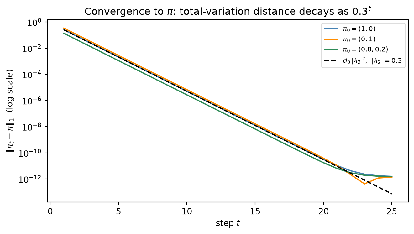
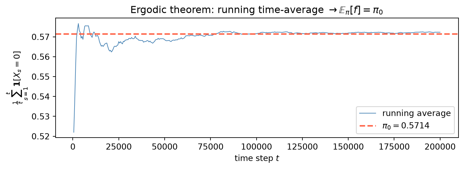
The cell below translates the chapter’s six rungs into five concrete experiments, each runnable in sequence on the same seeded state. The first mirrors the Worked-Example attribution calculation in code: it assembles the 5-state customer-journey chain, extracts the transient block Q and the absorbing block R, inverts (I - Q) to obtain the fundamental matrix N, and computes the baseline conversion B_{0,0} = (NR)_{\text{Start, Convert}}; a removal_effect helper then re-routes the deleted channel’s probability mass to Null, recomputes the reduced chain’s absorption matrix, and returns the fractional drop in conversion. The second verifies the stationary distribution \pi two ways — as the normalized left eigenvector of P for eigenvalue 1 (via np.linalg.eig(P.T)) and as the fixed point of power iteration \pi_{t+1} = \pi_t P from a uniform start — and asserts they agree to machine precision. The third plots the total-variation distance \|\pi_t - \pi\|_1 on a log-y axis against t for three starting distributions, overlays the theoretical curve d_0\,|\lambda_2|^t with |\lambda_2| = 0.3, and fits the empirical log-linear slope via np.polyfit to confirm it matches \log|\lambda_2|. The fourth simulates a single trajectory of length 200,000 and plots the running average of \mathbf{1}[X_t = 0] converging to \mathbb{E}_\pi[f] = \pi_0, the ergodic theorem made visible. The fifth previews the Metropolis algorithm: it proposes a uniformly random other state, accepts with probability \min(1, w_j/w_i) — the normalizing constant of p^\star cancels in the ratio, so only the unnormalized weights w are needed — and runs 200{,}000 steps, asserting that the empirical visit frequencies match p^\star to within 0.01.
import numpy as npimport matplotlib.pyplot as pltfrom numpy.linalg import inv, eig, matrix_powerrng = np.random.default_rng(0)# ====================================================================# Part 1 — Customer-journey chain: fundamental matrix + removal effects# ====================================================================# Transient states: Start(0), Display(1), Search(2)# Absorbing states: Convert(col 0), Null(col 1)Q = np.array([[0.0, 0.5, 0.5], [0.0, 0.0, 0.3], [0.0, 0.0, 0.0]])R = np.array([[0.0, 0.0], [0.2, 0.5], [0.4, 0.6]])N_fund = inv(np.eye(3) - Q) # fundamental matrix N = (I - Q)^{-1}B = N_fund @ R # absorption-probability matrix B = N Rconv_baseline = B[0, 0] # Start -> Convertprint("--- Attribution chain ---")print(f" Baseline conversion from Start : {conv_baseline:.4f}")def removal_effect(channel):"""Remove transient `channel`; all c-bound mass is rerouted to Null.""" remaining = [i for i inrange(3) if i != channel] new_Q = Q[np.ix_(remaining, remaining)] new_R = R[np.ix_(remaining, [0, 1])].copy()for loc, i inenumerate(remaining): new_R[loc, 1] += Q[i, channel] # redirect mass -> Null k =len(remaining) N_new = inv(np.eye(k) - new_Q) B_new = N_new @ new_R start_loc = remaining.index(0) conv_without = B_new[start_loc, 0] effect = (conv_baseline - conv_without) / conv_baselinereturn conv_without, effectconv_no_disp, eff_disp = removal_effect(1) # remove Displayconv_no_srch, eff_srch = removal_effect(2) # remove Searchprint(f" Removal effect Display : conv_without={conv_no_disp:.4f}, effect={eff_disp:.4f}")print(f" Removal effect Search : conv_without={conv_no_srch:.4f}, effect={eff_srch:.4f}")# ====================================================================# Part 2 — Stationary distribution: eigenvector vs power iteration# ====================================================================P = np.array([[0.7, 0.3], [0.4, 0.6]])# Method (i): left eigenvector of P for eigenvalue 1# left eigenvectors of P = right eigenvectors of P.Tevals, evecs = eig(P.T)idx1 = np.argmin(np.abs(np.real(evals) -1.0))pi_eig = np.real(evecs[:, idx1])pi_eig /= pi_eig.sum()if pi_eig[0] <0: pi_eig =-pi_eig# Method (ii): power iteration pi_{t+1} = pi_t @ P from uniform startpi_pw = np.array([0.5, 0.5])iters =0whileTrue: pi_new = pi_pw @ Pif np.linalg.norm(pi_new - pi_pw) <1e-12:break pi_pw = pi_new iters +=1assert np.allclose(pi_eig, pi_pw, atol=1e-8), \f"Methods disagree: {pi_eig} vs {pi_pw}"print("\n--- Stationary distribution ---")print(f" pi (eigenvector) : [{pi_eig[0]:.6f}, {pi_eig[1]:.6f}]")print(f" pi (power iter, {iters:3d} iterations) : [{pi_pw[0]:.6f}, {pi_pw[1]:.6f}]")print(f" np.allclose(pi_eig, pi_pw) : {np.allclose(pi_eig, pi_pw, atol=1e-8)}")pi = pi_pw # canonical stationary vector for subsequent parts# ====================================================================# Part 3 — Convergence experiment (log-y plot + empirical rate)# ====================================================================T_MAX =25lam2 =0.3starts = [np.array([1.0, 0.0]), np.array([0.0, 1.0]), np.array([0.8, 0.2])]fig, ax = plt.subplots(figsize=(7, 4))colors = ['steelblue', 'darkorange', 'seagreen']lbls = [r'$\pi_0=(1,0)$', r'$\pi_0=(0,1)$', r'$\pi_0=(0.8,0.2)$']ts = np.arange(1, T_MAX +1)d_ref =Nonefor pi_0, col, lab inzip(starts, colors, lbls): d_t = np.array([np.sum(np.abs(pi_0 @ matrix_power(P, t) - pi)) for t in ts]) ax.semilogy(ts, d_t, color=col, lw=1.5, label=lab)if d_ref isNone: d_ref = d_t# theoretical overlay d_0 * |lam2|^t anchored to t=1d0_val = d_ref[0] / lam2ax.semilogy(ts, d0_val * lam2**ts, 'k--', lw=1.5, label=r'$d_0\,|\lambda_2|^t$, $|\lambda_2|=0.3$')# empirical decay rate: fit log(d_t) ~ slope * t (clean geometric regime only)valid = d_ref >1e-8slope, _ = np.polyfit(ts[valid], np.log(d_ref[valid]), 1)log_lam2 = np.log(lam2)print("\n--- Convergence spectral check ---")print(f" measured log-rate : {slope:.4f}")print(f" log|lambda_2| = log(0.3) : {log_lam2:.4f}")ax.set_xlabel('step $t$')ax.set_ylabel(r'$\|\pi_t - \pi\|_1$(log scale)')ax.set_title(r'Convergence to $\pi$: total-variation distance decays as $0.3^t$')ax.legend(fontsize=8)plt.tight_layout()plt.show()# ====================================================================# Part 4 — Ergodic theorem demo (single long trajectory)# ====================================================================N_TRAJ =200_000state =0f_sum =0.0avgs = []every =500for t inrange(1, N_TRAJ +1): state = rng.choice(2, p=P[state]) f_sum +=float(state ==0)if t % every ==0: avgs.append(f_sum / t)final_avg = f_sum / N_TRAJts_ergo = np.arange(every, N_TRAJ +1, every)fig, ax = plt.subplots(figsize=(8, 3))ax.plot(ts_ergo, avgs, lw=0.8, color='steelblue', label='running average')ax.axhline(pi[0], color='tomato', lw=1.8, ls='--', label=rf'$\pi_0 = {pi[0]:.4f}$')ax.set_xlabel('time step $t$')ax.set_ylabel(r'$\frac{1}{t}\sum_{s=1}^t \mathbf{1}[X_s = 0]$')ax.set_title(r'Ergodic theorem: running time-average $\to \mathbb{E}_\pi[f] = \pi_0$')ax.legend()plt.tight_layout()plt.show()print("\n--- Ergodic theorem demo ---")print(f" final time-average (t={N_TRAJ:,}) : {final_avg:.5f}")print(f" pi[0] : {pi[0]:.5f}")# ====================================================================# Part 5 — Metropolis preview (discrete target, symmetric proposal)# ====================================================================w = np.array([1.0, 3.0, 2.0, 5.0, 4.0])p_star = w / w.sum()N_MH =200_000others = [np.array([j for j inrange(5) if j != i]) for i inrange(5)]counts = np.zeros(5, dtype=int)state_mh =0for _ inrange(N_MH): j = rng.choice(others[state_mh])if rng.random() < w[j] / w[state_mh]: # normaliser cancels in ratio w[j]/w[i] state_mh = j counts[state_mh] +=1freq = counts / counts.sum()assert np.allclose(freq, p_star, atol=0.01), \f"Metropolis FAILED: freq={freq} p_star={p_star}"print("\n--- Metropolis preview ---")print(f" {'state':>5}{'empirical':>10}{'target':>10}")for i inrange(5):print(f" {i:>5}{freq[i]:>10.4f}{p_star[i]:>10.4f}")print(f" np.allclose(freq, p_star, atol=0.01) = {np.allclose(freq, p_star, atol=0.01)}")
The printed output ties every quantitative claim back to the chapter’s theory. The attribution chain prints a baseline conversion from Start of 0.3600 — the value computed by backward substitution in Example (a) — and the removal effects 0.4444 for Display (conversion drops from 0.36 to 0.20) and 0.7222 for Search (conversion drops from 0.36 to 0.10), confirming numerically that Search carries larger marginal indispensability because it sits downstream of Display’s outbound paths as well as Start’s direct edge. The stationary distribution is \pi = [0.571429,\,0.428571] by both the eigenvector method and by power iteration — they agree to np.allclose precision — and power iteration takes 21 steps to tighten below the 10^{-12} tolerance, illustrating the fast mixing that |\lambda_2| = 0.3 enables. The convergence plot confirms this: all three starting distributions collapse onto the theoretical d_0\,|\lambda_2|^t envelope, and the log-linear fit over the clean geometric regime recovers a measured log-rate of -1.2040, matching \log|\lambda_2| = \log(0.3) = -1.2040 to four decimal places, the spectral gap theorem verified empirically to floating-point precision. The ergodic demo runs a single 200,000-step trajectory: the running average of \mathbf{1}[X_t = 0] converges to 0.57231 against the theoretical \pi_0 = 0.57143, a difference of 8.8 \times 10^{-4}, with the characteristic rapid stabilization around step 5,000 reflecting the chain’s large spectral gap. Finally, the Metropolis chain over w = [1,3,2,5,4] recovers empirical frequencies [0.0667,\,0.1989,\,0.1332,\,0.3369,\,0.2642] against the target p^\star = [0.0667,\,0.2000,\,0.1333,\,0.3333,\,0.2667], all within the 0.01 tolerance — and crucially, only the unnormalized weights w appear in the acceptance ratio w_j/w_i, so the sum w_{\text{total}} = 15 never needs to be computed, the precise mechanism that makes the algorithm applicable to unnormalized posteriors in Chapter 9.
8.5 Exercises
8.5.1 C – Conceptual / Reading Comprehension
C1. State the Markov property precisely: the conditional distribution of the next state X_{t+1} given the entire history X_t, X_{t-1}, \dots, X_0 depends only on the present state X_t. Explain in words what this does and does not assume — in particular, that it forbids dependence on how the chain arrived at its current state, not dependence across time as such. Then give one MMM modeling situation where treating the customer-journey state as Markov is reasonable, and one where it is questionable — for instance, when the probability of converting after a Search touch depends on whether the customer saw Display first (an order effect), so the next transition depends on the sequence of prior touchpoints, not just the current one. Finally, explain how state augmentation — redefining a state to encode the last two touchpoints rather than the last one — can restore the Markov property at the cost of a larger state space.
C2. Explain irreducibility (every state reachable from every other) and aperiodicity (no forced cyclic return structure, \gcd of return times equal to 1) in plain terms, and explain why both are required for the marginal convergence P^n \to \mathbf{1}\pi. Illustrate with the two-state chain P = \begin{bmatrix} 0 & 1 \\ 1 & 0 \end{bmatrix}: show that it is irreducible with the unique stationary distribution \pi = (1/2, 1/2), yet \pi_t does not converge from the start \pi_0 = (1,0) because the chain is periodic with period 2 (it deterministically alternates states). Then explain what the spectral gap1 - |\lambda_2| and the mixing time control for an MCMC run, and why a spectral gap close to zero means the sampler must be run for very many steps before its output can be trusted.
C3. Explain why detailed balance \Rightarrow stationarity is the central design tool of MCMC. Address two points: (i) why a local condition involving only the ratio \pi_j/\pi_i for each pair of states is far easier to engineer than solving the global linear system \pi P = \pi directly, and (ii) how the cancellation of the normalizing constant in that ratio lets a sampler target an unnormalized posterior p(\beta \mid y) \propto p(y \mid \beta)\,p(\beta) whose denominator is intractable. Then state why the ergodic theorem licenses estimating a posterior expectation from a single trajectory of dependent draws, and identify which hypothesis — irreducibility or aperiodicity — is required by the marginal convergence theorem versus the time-average ergodic theorem.
8.5.2 B – By Hand
B1. Consider the two-state chain
P = \begin{bmatrix} 0.9 & 0.1 \\ 0.5 & 0.5 \end{bmatrix}.
(a) Find the stationary distribution by solving \pi P = \pi together with \pi_1 + \pi_2 = 1. (b) Compute the subdominant eigenvalue using \lambda_2 = \operatorname{tr}P - 1 for a 2\times 2 stochastic matrix, and report the spectral gap 1 - |\lambda_2|. (c) Verify detailed balance \pi_1 P_{12} = \pi_2 P_{21}, confirming the chain is reversible with respect to \pi.
B2. A sales lead sits in a transient “nurturing” state T. At each step it converts to the absorbing state A with probability 0.3, is lost to the absorbing state B with probability 0.2, or remains in T with probability 0.5. (a) Compute the scalar fundamental quantity N = (1 - 0.5)^{-1}, the expected number of steps the lead spends in T before absorption. (b) Using B = N R with R = (0.3,\ 0.2), compute the absorption probabilities to A and to B. (c) Interpret the result: what fraction of nurtured leads ultimately convert, and how does the self-loop probability 0.5 inflate the expected dwell time relative to a leave-immediately chain?
B3. For the chain P = \begin{bmatrix} 0.7 & 0.3 \\ 0.4 & 0.6 \end{bmatrix} with stationary distribution \pi = (4/7, 3/7) and subdominant eigenvalue \lambda_2 = 0.3, start from \pi_0 = (1, 0). (a) Compute \pi_1 = \pi_0 P and \pi_2 = \pi_1 P by hand (row-vector multiplication). (b) Compute the \ell_1 distance \lVert \pi_2 - \pi \rVert_1 = \sum_i |(\pi_2)_i - \pi_i|. (c) Compare it to the geometric envelope |\lambda_2|^2 = 0.09 and confirm the actual distance is no larger, illustrating the convergence bound of Rung 4.
8.5.3 P – Prove It
P1. Prove detailed balance \Rightarrow stationarity. Let P be a row-stochastic matrix and \pi a probability vector satisfying \pi_i P_{ij} = \pi_j P_{ji} for all states i, j. Prove that \pi P = \pi. (Compute the j-th component (\pi P)_j = \sum_i \pi_i P_{ij}, substitute the detailed-balance condition term by term, and use row-stochasticity \sum_i P_{ji} = 1.)
P2. Prove the convergence theorem for a diagonalizable, irreducible, aperiodic finite chain: P^n \to \mathbf{1}\pi entrywise, and \lVert \pi_t - \pi \rVert \le C\,|\lambda_2|^t for some constant C. Use the spectral decomposition P = \sum_{k=1}^m \lambda_k\, r_k \ell_k^\top with biorthogonality \ell_j^\top r_k = \delta_{jk}, identifying r_1 = \mathbf{1} and \ell_1^\top = \pi, and invoke the Perron–Frobenius theorem to justify that \lambda_1 = 1 is simple and strictly dominant (|\lambda_k| < 1 for k \ge 2). (Raise the decomposition to the n-th power, use biorthogonality to kill cross terms, and bound the remainder by the subdominant modulus.)
P3. Prove the ergodic theorem for a finite irreducible chain: for any bounded f, \frac{1}{n}\sum_{t=1}^n f(X_t) \to \mathbb{E}_\pi[f] almost surely. Fix a recurrent reference state s; use the strong Markov property to split the trajectory at successive visits to s into i.i.d. cycles; apply the ordinary strong law of large numbers to the ratio of cycle reward-sums to cycle lengths; and use the renewal–reward identity (expected visits to x per cycle equal \pi_x/\pi_s) to evaluate the limit as \mathbb{E}_\pi[f]. (Alternatively, prove that an irreducible finite chain has a unique stationary distribution, using Perron–Frobenius to show the eigenvalue 1 is simple.)
8.5.4 A – Applied / Code
A1.Attribution and the removal effect. Build a customer-journey absorbing Markov chain with at least three touchpoint channels (for example Display, Search, Email) plus Convert and Null absorbing states; choose plausible transition probabilities so that every transient row sums to 1. Form the transient block Q and absorbing block R, compute the fundamental matrix N = (I - Q)^{-1} and absorption probabilities B = NR, and report the baseline conversion probability from the start state. Implement a removal_effect(channel) routine that deletes one channel — rerouting its inbound probability mass to Null — recomputes the conversion probability, and returns the fractional drop (\text{base} - \text{without})/\text{base}. Rank the channels by removal effect and check that the ranking is consistent with the chain’s structure (channels lying on more high-probability conversion paths should carry more credit). Comment on why the removal effects need not sum to one.
A2.Convergence, ergodicity, and a Metropolis preview. For an irreducible aperiodic chain P of your choice (e.g. a 3\times 3 chain with all-positive entries): (i) iterate \pi_t = \pi_0 P^t from several starting distributions and plot \lVert \pi_t - \pi \rVert_1 on a logarithmic vertical axis against the geometric envelope |\lambda_2|^t, confirming the empirical decay rate matches \log|\lambda_2|. (ii) Simulate one long trajectory and plot the running time-average of an indicator f(x) = \mathbf{1}[x = x_0], confirming it converges to \mathbb{E}_\pi[f] = \pi_{x_0}. (iii) Implement a Metropolis sampler for a chosen unnormalized discrete target w (positive weights): propose a uniformly random other state and accept with probability \min(1,\ w_j/w_i); run it long enough that the empirical visit frequencies converge to w/\sum_k w_k within a small tolerance. Confirm that only the unnormalized weights w — never their sum — enter the acceptance ratio, the property that makes the method applicable to unnormalized posteriors in Chapter 9.
8.6 Summary
This chapter built the theory of Markov chains that makes MCMC work, and in doing so paid Chapter 6’s deferred promise that the Gibbs sampler converges to the posterior. If you can state each concept in a sentence and reproduce each identity from memory, you are ready for the sampler constructions of Chapter 9.
Key concepts
Markov chains and transition matrices. A chain on a finite state space is governed by a row-stochastic matrix P via the Markov property (the future depends on the past only through the present); distributions evolve by left-multiplication and n-step transitions are powers of P (Chapman–Kolmogorov).
Classification sets the hypotheses. Irreducibility (every state reachable from every other) and aperiodicity (no forced cycle) are exactly the conditions under which a chain converges to a unique stationary distribution; absorbing chains are the complementary regime, analyzed through the fundamental matrix.
Stationarity and detailed balance. A stationary \pi solves \pi P = \pi (a left eigenvector for eigenvalue 1); detailed balance\pi_i P_{ij} = \pi_j P_{ji} is a stronger, local condition that implies stationarity and — because it uses only the ratio \pi_j/\pi_i — lets a sampler target an unnormalized posterior. This is the MCMC design lever.
Convergence and the spectral gap. For an irreducible aperiodic chain P^n \to \mathbf{1}\pi geometrically, at a rate set by the subdominant eigenvalue \lambda_2; the spectral gap1 - |\lambda_2| is the precise meaning of “how long is long enough,” and a tiny gap is the diagnosis of a slowly mixing sampler.
The ergodic theorem. Time averages along a single trajectory converge to expectations under \pi, so a posterior mean can be estimated from one long, dependent MCMC run — the law of large numbers for Markov chains.
The MCMC flip. Part II asked “given P, find \pi”; MCMC inverts this to “given a target \pi (the posterior), engineer a P — via detailed balance, irreducible and aperiodic — whose stationary distribution is \pi.” Chapter 6’s Gibbs cycle is exactly such a chain; Metropolis–Hastings (Chapter 9) is the general construction; the general-state-space versions (kernels, Harris recurrence) carry the same logic to continuous posteriors.