Theory & Proofs
The diagnostics of Part A form a ladder. Rung 1 quantifies the residual error that survives even at stationarity — the finite-sample noise in any quantity computed from the draws. Rung 2 builds the convergence statistic \hat{R} that certifies stationarity itself, with a full proof of why it tends to one when the chains agree and exceeds one when they do not, then sharpens it into the split and rank-normalized forms used in practice. Rung 3 (next) defines the effective sample size that Rung 1 already needs. Before the rungs, we fix the running model on which every diagnostic will be exercised.
The running model
Every diagnostic in this chapter is developed on a single small hierarchical model — the one on which essentially the entire MCMC-diagnostics literature was first worked out. The eight-schools model (Gelman et al. 2013) estimates the effect of a coaching program in J = 8 schools. For school j, a separate analysis produced a noisy estimate y_j of the true effect \theta_j, with a known standard error \sigma_j:
y_j \mid \theta_j \sim \mathcal{N}(\theta_j,\, \sigma_j^2), \qquad
\theta_j \mid \mu, \tau \sim \mathcal{N}(\mu,\, \tau^2), \qquad j = 1, \dots, J.
The school-level effects \theta_j are drawn from a common population \mathcal{N}(\mu, \tau^2), with weak priors placed on the population mean \mu and the between-school standard deviation \tau. The \sigma_j are known measurement standard errors; \mu is the population mean effect, and \tau governs how much the \theta_j are pulled toward \mu — full pooling as \tau \to 0, no pooling as \tau \to \infty.
Same math, marketing labels. Read \theta_g as a geo-level effect — the incremental ROAS, or the baseline sales level, of region g — partially pooled toward a national mean \mu with cross-geo standard deviation \tau. The observation y_g is that geo’s noisy regression estimate of the effect, carrying a standard error \sigma_g inherited from the geo-level fit. The structure is identical to eight schools; only the nouns change. And so does the trap: when only a handful of geos are available, \tau is weakly identified, and a weakly identified \tau reproduces exactly the funnel geometry of Chapter 10 — the variance parameter and its dependent effects squeezing into a narrow neck — which the sampler announces as divergences. The diagnostics below are precisely the instruments that catch this.
Rung 1 — Monte Carlo standard error
A posterior summary is never computed from the posterior itself; it is computed from a finite sample of draws, and so it carries its own sampling error on top of whatever uncertainty the posterior already expresses. Reporting the summary without that error is reporting a measurement without its tolerance.
Let \theta^{(1)}, \dots, \theta^{(N)} be the draws of a scalar quantity from a converged chain, and consider the ergodic average
\widehat{\mathbb{E}}[\theta] = \frac{1}{N}\sum_{i=1}^{N} \theta^{(i)},
our estimate of the posterior mean \mathbb{E}[\theta]. The Markov-chain central limit theorem of Chapter 9 tells us this estimate is asymptotically normal around the true mean, with a standard error
\text{MCSE} = \frac{\sigma_\theta}{\sqrt{N_{\text{eff}}}},
where \sigma_\theta is the posterior standard deviation of \theta and N_{\text{eff}} is the effective sample size — the number of independent draws that would carry the same information as the N correlated draws actually in hand (constructed in Rung 3). The form mirrors the classical \sigma/\sqrt{N}, but with N replaced by N_{\text{eff}}.
The replacement is the whole point. Successive draws of a Markov chain are autocorrelated: each draw is a perturbation of the last, not a fresh sample, so a run of N draws carries less information than N independent samples would. Autocorrelation inflates the variance of the ergodic average, and the inflation is absorbed by setting N_{\text{eff}} < N. A chain that mixes well has N_{\text{eff}} close to N; a sticky chain that crawls along a posterior ridge can have N_{\text{eff}} orders of magnitude smaller, and its summaries are correspondingly noisier than their draw count suggests.
The practical rule is simple: report MCSE alongside every posterior summary, and quote the summary only to the precision the MCSE supports. An MMM that reports a channel’s ROAS as 2.47 when the MCSE is 0.05 is claiming a third significant figure that the sampler never resolved — false precision that an optimizer will nonetheless treat as exact. If the MCSE bites the second figure, the second figure should not be printed.
Rung 2 — The Gelman–Rubin statistic \hat{R}
MCSE presumes convergence; the next diagnostic tests for it. The idea behind the Gelman–Rubin statistic is to run several chains from overdispersed starting points and ask whether they have forgotten where they began. If every chain has converged to the same target, the variation between chains should be no larger than the variation within each chain. If the chains are still wandering in separate regions, the between-chain variation will dominate. \hat{R} makes this comparison a single number.
Run M chains, each of length N, on a scalar quantity \theta. Let \bar\theta_m be the mean of chain m, let \bar\theta = \frac{1}{M}\sum_{m=1}^{M}\bar\theta_m be the grand mean, and let s_m^2 be the within-chain sample variance of chain m. Define the between-chain and within-chain variance estimates
B = \frac{N}{M-1}\sum_{m=1}^{M}(\bar\theta_m - \bar\theta)^2, \qquad
W = \frac{1}{M}\sum_{m=1}^{M} s_m^2,
and combine them into the marginal posterior variance estimate and the statistic itself:
\widehat{\operatorname{var}}^+(\theta) = \frac{N-1}{N}W + \frac{1}{N}B, \qquad
\hat{R} = \sqrt{\frac{\widehat{\operatorname{var}}^+(\theta)}{W}}.
Theorem (\hat{R} detects non-convergence). If the M chains are stationary and have converged to a common target with finite variance, then \hat{R} \to 1 as N \to \infty. If the chains have not mixed — if they occupy systematically different regions of parameter space — then \hat{R} > 1.
Proof. Converged case. Suppose first that all chains have converged to the common target, whose marginal variance for \theta is \operatorname{var}(\theta).
The within-chain term W averages the M within-chain sample variances. Each s_m^2 is a consistent estimator of the marginal variance of a stationary chain, so as N \to \infty each s_m^2 \to \operatorname{var}(\theta) and therefore
W \to \operatorname{var}(\theta).
For the between-chain term, note that B/N = \frac{1}{M-1}\sum_{m=1}^{M}(\bar\theta_m - \bar\theta)^2 is the sample variance of the M chain means. For converged chains the means \bar\theta_m are independent and identically distributed, each an average of N stationary draws, so \operatorname{var}(\bar\theta_m) = \operatorname{var}(\theta)/N (up to the autocorrelation correction, which does not change the scaling). Hence B/N estimates \operatorname{var}(\theta)/N, giving
B \to \operatorname{var}(\theta), \qquad \frac{B}{N} \to 0.
Combining the two limits in the marginal variance estimate,
\begin{aligned}
\widehat{\operatorname{var}}^+(\theta)
&= \frac{N-1}{N}\,W + \frac{1}{N}\,B \\
&\to 1 \cdot \operatorname{var}(\theta) + 0 \\
&= \operatorname{var}(\theta),
\end{aligned}
since (N-1)/N \to 1 and B/N \to 0. Therefore
\hat{R} = \sqrt{\frac{\widehat{\operatorname{var}}^+(\theta)}{W}}
\to \sqrt{\frac{\operatorname{var}(\theta)}{\operatorname{var}(\theta)}} = 1.
Unmixed case. Now suppose the chains have not mixed: they sit in systematically different regions, so the chain means \bar\theta_m differ by amounts that do not shrink as N grows. Then B, which scales those squared mean differences by N, does not vanish on the relative scale, and \widehat{\operatorname{var}}^+(\theta) — built to be unbiased only under the overdispersed-initialization assumption that the chains jointly cover the target — overestimates \operatorname{var}(\theta). At the same time each chain, confined to its own region, explores only part of the target, so W underestimates \operatorname{var}(\theta). The ratio therefore exceeds one,
\hat{R} = \sqrt{\frac{\widehat{\operatorname{var}}^+(\theta)}{W}} > 1,
and remains bounded away from one until the chains overlap. \blacksquare
The classical advice was to accept convergence once \hat{R} < 1.1. Modern practice is stricter: declare non-convergence unless \hat{R} < 1.01 (Vehtari et al. 2021), because the looser threshold lets through chains whose residual bias is large enough to corrupt tail estimates and MCSE.
The plain statistic above has two blind spots, each closed by a refinement.
Split-\hat{R}. A single chain that drifts steadily — never settling, but moving slowly enough that its overall mean still resembles the others’ — can pass the whole-chain test while being plainly non-stationary. Split-\hat{R} catches this by cutting each chain into its first and second halves and treating the 2M halves as separate chains before computing \hat{R}. A drifting chain has mismatched halves, which inflates the between-chain term and exposes the non-stationarity that the undivided statistic concealed (Vehtari et al. 2021).
Rank-normalized \hat{R}. The variance-based statistic presumes the target has a finite variance; for a heavy-tailed posterior — and an MMM ROAS posterior can be heavy-tailed — \operatorname{var}(\theta) may be enormous or undefined, and \hat{R} becomes unstable or meaningless. The fix is to replace each draw by the normal score of its rank across all chains and all draws, then compute \hat{R} on these rank-normalized values. Ranks are always finite, so the transformed quantity has a well-defined variance and the diagnostic stays valid even for heavy-tailed or infinite-variance targets (Vehtari et al. 2021). The split and rank-normalized refinements are applied together, and their combination is the \hat{R} that Stan and PyMC report by default.
Rung 3 — Effective sample size
Rung 1 wrote the Monte Carlo standard error as \sigma_\theta/\sqrt{N_{\text{eff}}} and then deferred the definition of N_{\text{eff}} to here. The deferral was not evasion: the effective sample size cannot be read off the draws one at a time, because it is a property of how the draws relate to one another. It is built from the autocorrelation structure of the chain — the same structure Chapter 9 introduced as the cost of dependent sampling — and the construction is a single theorem about the variance of a correlated average.
Theorem (variance inflation). For a stationary sequence \theta^{(1)}, \dots, \theta^{(N)} with marginal variance \sigma^2 and lag-k autocorrelation \rho_k = \operatorname{corr}(\theta^{(i)}, \theta^{(i+k)}), the variance of the sample mean is
\operatorname{var}(\bar\theta) = \frac{\sigma^2}{N}\left(1 + 2\sum_{k=1}^{N-1}\Bigl(1 - \frac{k}{N}\Bigr)\rho_k\right),
and as N \to \infty this tends to \frac{\sigma^2}{N}\bigl(1 + 2\sum_{k=1}^{\infty}\rho_k\bigr). The effective sample size is therefore
N_{\text{eff}} = \frac{N}{1 + 2\sum_{k=1}^{\infty}\rho_k}.
Proof. Begin from the variance of the sample mean written as a double sum over all pairs of draws:
\operatorname{var}(\bar\theta) = \operatorname{var}\!\left(\frac{1}{N}\sum_{i=1}^{N}\theta^{(i)}\right) = \frac{1}{N^2}\sum_{i=1}^{N}\sum_{j=1}^{N}\operatorname{cov}(\theta^{(i)}, \theta^{(j)}).
By stationarity the covariance between two draws depends only on the lag between them: \operatorname{cov}(\theta^{(i)}, \theta^{(j)}) = \sigma^2 \rho_{|i-j|}, with \rho_0 = 1. Group the N^2 pairs by their lag k = |i - j|. The N diagonal pairs (i = j) contribute lag 0; for each lag k = 1, \dots, N-1 there are exactly 2(N-k) ordered pairs (i, j) with |i - j| = k — the factor of two counting i < j and i > j separately. Hence
\begin{aligned}
\operatorname{var}(\bar\theta)
&= \frac{1}{N^2}\left(N\sigma^2 + \sum_{k=1}^{N-1} 2(N-k)\,\sigma^2 \rho_k\right) \\
&= \frac{\sigma^2}{N^2}\left(N + 2\sum_{k=1}^{N-1}(N-k)\,\rho_k\right) \\
&= \frac{\sigma^2}{N}\left(1 + 2\sum_{k=1}^{N-1}\Bigl(1 - \frac{k}{N}\Bigr)\rho_k\right),
\end{aligned}
which is the finite-N formula. As N \to \infty the triangular weights 1 - k/N \to 1 for each fixed lag k; assuming the autocorrelations are summable, \sum_k |\rho_k| < \infty, the weighted sum converges to \sum_{k=1}^{\infty}\rho_k and
\operatorname{var}(\bar\theta) \;\to\; \frac{\sigma^2}{N}\left(1 + 2\sum_{k=1}^{\infty}\rho_k\right).
Finally, define N_{\text{eff}} by demanding that the correlated average have the same variance as an average of N_{\text{eff}} independent draws, \operatorname{var}(\bar\theta) = \sigma^2/N_{\text{eff}}. Matching the two expressions and solving gives
N_{\text{eff}} = \frac{N}{1 + 2\sum_{k=1}^{\infty}\rho_k}. \qquad \blacksquare
The denominator has a name: the integrated autocorrelation time \tau_{\text{int}} = 1 + 2\sum_{k\ge 1}\rho_k, so that N_{\text{eff}} = N/\tau_{\text{int}}. This closes the loop with Rung 1: substituting back, the MCSE is \sigma_\theta/\sqrt{N_{\text{eff}}} = \sigma_\theta\sqrt{\tau_{\text{int}}/N}, and the autocorrelation time is exactly the factor by which dependence inflates the Monte Carlo error above the i.i.d. baseline \sigma_\theta/\sqrt{N}.
A worked AR(1) case fixes intuition. For a first-order autoregressive chain with lag-1 autocorrelation \phi = 0.5, the autocorrelations decay geometrically, \rho_k = \phi^k, so the integrated time is a single geometric series:
\tau_{\text{int}} = 1 + 2\sum_{k\ge1}\phi^k = 1 + 2\cdot\frac{\phi}{1-\phi} = 1 + 2\cdot\frac{0.5}{0.5} = 3.
A run of N such draws is worth only N/3 independent ones — ten thousand iterations carry the information of roughly three thousand. Push \phi toward one, the regime of a sticky chain crawling along a posterior ridge, and \tau_{\text{int}} diverges while N_{\text{eff}} collapses, exactly the pathology Chapter 9 traced to collinear channel spend.
Bulk-ESS versus tail-ESS. A single effective sample size is not enough, because different posterior summaries draw on different parts of the distribution (Vehtari et al. 2021). Bulk-ESS is computed on the rank-normalized draws and governs estimates of central tendency — the posterior mean and median. Tail-ESS is computed from the indicator series for the 5\% and 95\% quantiles and governs the reliability of the interval endpoints. The two can diverge sharply: a chain may have ample bulk-ESS, so its point estimate is well resolved, yet poor tail-ESS, so its credible-interval bounds are noisy. Reporting one number hides this. For an MMM ROAS the credible interval is often what drives the decision — whether a channel’s lower bound clears the cost of capital — so tail-ESS matters every bit as much as bulk, and both should be checked before a posterior interval is trusted.
Rung 4 — Divergences and the energy diagnostics
\hat{R} and effective sample size are necessary but not sufficient. Both are computed from the draws the sampler actually collected, and so both are silent about the draws it never collected. A chain can post a perfect \hat{R} and a generous ESS while an entire region of the posterior — the narrow neck of a hierarchical funnel — goes wholly unvisited, because the statistics summarize only the territory already explored. Detecting the unexplored requires diagnostics that look not at the draws but at the geometry the sampler is moving through. Hamiltonian Monte Carlo, which simulates physical trajectories across that geometry, supplies exactly such diagnostics.
Divergences. A divergent transition is one in which the leapfrog integrator’s energy error explodes (Chapter 10). The simulated Hamiltonian trajectory should conserve energy exactly; when the step size is too coarse to resolve a region of high curvature — the funnel neck, where the posterior pinches as \tau \to 0 and the dependent effects are squeezed into a sliver — the discretized dynamics instead fly apart, and the energy of the simulated path diverges from its starting value. The sampler flags the transition and refuses to follow it. Even a handful of divergences is a warning, not a nuisance: it means the sampler is systematically avoiding a part of the posterior it cannot integrate through, so the draws it returns are biased toward the regions it can reach, not merely noisier than their count suggests. This is a geometry alarm, not a convergence statistic. It can fire while \hat{R} and ESS look immaculate, precisely because those statistics never inspect the territory the divergences mark as missing (Betancourt 2017).
BFMI (energy Bayesian fraction of missing information). Where divergences probe local curvature, the energy diagnostic probes global exploration. Between trajectories, HMC resamples the momentum and thereby moves the chain from one energy level to another; the BFMI measures how effectively that resampling explores the marginal distribution of the energy. A low BFMI means successive energy levels are too similar — the momentum refreshment is not carrying the chain across the full range of energies the posterior occupies — so the sampler cannot reach the tails efficiently. It is a flag for slow mixing in the heavy-tailed directions, the directions where an MMM’s weakly identified variance parameters live (Betancourt 2017).
Tree-depth saturation (NUTS). The No-U-Turn Sampler grows each trajectory until a U-turn criterion signals that continuing would double back, subject to a maximum tree depth that caps the work per iteration. When NUTS repeatedly hits that maximum, its trajectories are being truncated before the U-turn would naturally stop them: the sampler is exploring correctly but is cut short, taking many small, expensive steps where a longer trajectory would have moved farther for less cost. This is an efficiency alarm, not a bias alarm — the draws are valid, just dearer than they should be.
The three signals partition cleanly. Divergences are a bias alarm; BFMI and tree-depth saturation are efficiency alarms. A bias alarm says the answer may be wrong; an efficiency alarm says the answer is right but costlier than necessary. This is why the convergence diagnostics of Rungs 2 and 3 (\hat{R}, ESS) and the geometric diagnostics of this rung (divergences above all) are complementary rather than redundant: the former certify that the draws you have are a faithful sample of where the chain went, the latter warn when where the chain went is not where the posterior actually lives. A trustworthy MMM fit must clear both.
Everything to this point has been Part A: it certified that the sampler faithfully characterized the posterior of a model, that the draws in hand are a trustworthy sample from p(\theta \mid y). It said nothing about whether that model deserves belief. A perfectly converged fit of a badly specified model is a precise answer to the wrong question. Part B asks instead: is the model any good? — and it splits in two. B1, self-consistency: does the model reproduce the data it was fit to, and are the intervals it reports honest? This is the work of predictive checks and simulation-based calibration, Rungs 5 through 7. B2, out-of-sample prediction: does the model generalize to data it has not seen? — taken up later. The next two rungs build the predictive checks that anchor B1.
Rung 5 — Predictive checks
A model is a generative claim: it asserts that data arise from a particular stochastic process. The most direct test of such a claim is to run the process and look at what comes out — before fitting, to audit the priors, and after fitting, to audit the fit.
Prior predictive checks. Before any data touches the model, draw a parameter vector from the prior, \theta \sim p(\theta), then a dataset from the likelihood given that draw, \tilde{y} \sim p(y \mid \theta). Repeating this traces out the prior predictive distribution
p(\tilde{y}) = \int p(\tilde{y} \mid \theta)\,p(\theta)\,d\theta,
the distribution of datasets the model considers plausible before seeing any data. The check is to inspect whether these simulated datasets are remotely reasonable — the right order of magnitude, the right sign, a sensible range. This is cheap and it catches absurd priors before a single expensive MCMC run is launched. In an MMM the payoff is concrete: a prior that lets a single channel’s contribution exceed total observed sales by an order of magnitude is exposed immediately in the prior predictive draws, not discovered after a week of sampling, divergence-chasing, and debugging a fit that was doomed by its priors from the start.
Posterior predictive checks (PPC). After fitting, the analogous object conditions on the data. The posterior predictive distribution is
p(y^{\text{rep}} \mid y) = \int p(y^{\text{rep}} \mid \theta)\,p(\theta \mid y)\,d\theta,
the distribution of replicated datasets the fitted model would generate. It is sampled in two stages that mirror the prior predictive, with the posterior in place of the prior: draw \theta^{(s)} \sim p(\theta \mid y) from the posterior, then y^{\text{rep},(s)} \sim p(\cdot \mid \theta^{(s)}) from the likelihood. Because the posterior draws are already in hand from the MCMC run, the replicates cost only a forward simulation apiece.
The check turns on a test quantity T(y, \theta) — a scalar summary chosen to be sensitive to a feature of the data you care about: the maximum, the minimum, a count of zeros, a discrepancy between two groups. Compare the observed value to the distribution of the quantity over replicates. If the observed data is typical of what the model generates, the replicate distribution of T will be centered near the observed value and the model reproduces that feature; if T(y) sits in the extreme tail of the replicate distribution, the model cannot generate data with that feature and the misfit is exposed. The discipline is to pick test quantities that probe the failure modes that would actually hurt the decision — for an MMM, the size of the largest weekly sales spike, or the share of weeks with near-zero spend on a channel — rather than the features the model is guaranteed to fit by construction (Gelman et al. 2013).
This comparison is summarized by the posterior predictive p-value, the tail probability of the observed test quantity under the replicate distribution:
p_B = \Pr\!\bigl(T(y^{\text{rep}}, \theta) \ge T(y, \theta) \,\big|\, y\bigr),
estimated as the fraction of posterior-predictive replicates whose test quantity equals or exceeds the observed value. A p_B near 0 or 1 flags a feature the model systematically under- or over-produces; the question is what value p_B should take when the model is correct, which is the subject of the next rung.
Rung 6 — When is a p-value honest? The probability integral transform
A predictive p-value is only interpretable if we know what distribution it follows under a correct model — otherwise an observed value of, say, 0.05 has no reference against which to be judged surprising. For a continuous test statistic the answer is clean and universal: under a correct model the p-value is uniform on [0, 1]. The reason is a single fact about cumulative distribution functions, the probability integral transform.
Proposition (PIT uniformity). Let T be a continuous test statistic with cumulative distribution function F under the (correct) model. Then the random variable U = F(T) is uniformly distributed on [0, 1]. Consequently, if the model is correct, the tail probability p_B is \text{Uniform}(0,1).
Proof. Fix u \in [0,1]. Using that F is continuous and nondecreasing with (generalized) inverse F^{-1},
\begin{aligned}
\Pr(U \le u) &= \Pr(F(T) \le u) && \text{(definition $U = F(T)$)} \\
&= \Pr(T \le F^{-1}(u)) && \text{($F$ nondecreasing)} \\
&= F(F^{-1}(u)) && \text{(definition of $F$)} \\
&= u, && \text{($F \circ F^{-1} = \mathrm{id}$)}
\end{aligned}
which is exactly the cumulative distribution function of \text{Uniform}(0,1). Hence U \sim \text{Uniform}(0,1). \blacksquare
The practical reading follows directly. Under a correct model the p-value is uniform, so systematic departure from uniformity — a pile-up of p-values near 0, near 1, or bunched in the middle — is evidence of misfit, and the shape of the departure points to its kind. By the same token a single p-value near 0.5 is weak evidence: it is consistent with a correct model, but it is equally consistent with a great many wrong ones, and on its own it certifies nothing.
There is a crucial caveat, and it is structural rather than incidental. The posterior predictive p-value uses the data twice — once to fit the posterior p(\theta \mid y), and again to test against it through T(y, \theta). Because the replicate distribution is generated from a posterior that was itself pulled toward the observed data, the replicates are pulled toward y as well, and p_B is biased toward 0.5. The check is therefore conservative: it is less sensitive than its uniform ideal, more apt to pass a misspecified model than the clean PIT result would suggest. This double-use of the data is exactly the defect that simulation-based calibration removes, by working in the prior-predictive space — where parameters and data are drawn jointly and no datum is reused — rather than conditioning on a single observed dataset. That construction is the subject of Rung 7.
Rung 7 — Simulation-based calibration
Rung 6 closed on a debt. The posterior predictive p-value is conservative because it spends the observed data twice — once to build the posterior, once to test it — and a check that grades its own homework against the answer key can only ever be lenient. Simulation-based calibration (SBC) settles that debt by refusing to condition on any single observed dataset at all. It works entirely in the prior-predictive space, where a parameter and a dataset are drawn jointly from the model’s own generative process and nothing is reused: the truth comes first, the data follow from it, and the inference is then asked to recover the truth it was never told. The payoff is a validation of the entire inference procedure — the model, the algorithm, and the particular implementation of both — against a signal that is exact, distribution-free, and the same for every model: a uniform distribution of ranks (Talts et al. 2018).
The construction
Fix a scalar parameter \theta; the vector case applies the construction coordinatewise, one rank per component. A single SBC replication runs four steps.
- Draw a ground-truth parameter from the prior, \theta_0 \sim p(\theta).
- Draw a dataset from the likelihood at that truth, y \sim p(y \mid \theta_0).
- Run the inference under test on y to obtain L posterior samples \theta_1, \dots, \theta_L \sim p(\theta \mid y).
- Compute the rank statistic
r = \#\{\ell : \theta_\ell < \theta_0\} \in \{0, 1, \dots, L\},
the number of posterior draws that fall below the ground truth.
The claim that turns this into a test is that a single number — the rank — carries a known, model-independent distribution whenever the inference is exact.
The theorem and its proof
Theorem (SBC rank uniformity). If the inference is exact — the \theta_\ell are genuine draws from the true posterior p(\theta \mid y) — then over the joint generation of (\theta_0, y, \theta_{1:L}) the rank statistic r is uniformly distributed on \{0, 1, \dots, L\}.
Proof. The argument has three steps: the data-averaged posterior is the prior; therefore the truth and each posterior draw share that prior as their marginal law; therefore the L+1 values are exchangeable, and the rank of an exchangeable value is uniform.
Step 1 — the data-averaged posterior equals the prior. Let p(y) = \int p(y \mid \theta')\,p(\theta')\,d\theta' be the prior-predictive (marginal likelihood). Averaging the posterior over datasets drawn from this marginal returns the prior:
\begin{aligned}
\int p(\theta \mid y)\,p(y)\,dy
&= \int p(\theta, y)\,dy \\
&= p(\theta).
\end{aligned}
The first equality is Bayes’ rule read backwards — p(\theta \mid y)\,p(y) = p(\theta, y) is precisely the joint density — and the second is the definition of a marginal: integrating the joint over y removes y and leaves the prior marginal p(\theta). The posterior, weighted by how often each dataset actually occurs under the model, reconstructs the prior exactly.
Step 2 — the truth and the posterior draws are identically distributed. In the SBC generative process the truth is drawn \theta_0 \sim p(\theta) and the data y \sim p(y \mid \theta_0), so the pair (\theta_0, y) has joint density p(\theta_0, y) = p(y \mid \theta_0)\,p(\theta_0), and the marginal law of \theta_0 is the prior p(\theta) by construction. A posterior draw \theta_\ell is generated by first producing y through that same process and then sampling \theta_\ell \sim p(\theta \mid y). Its marginal density, averaged over the whole process, is therefore
\int p(\theta_\ell \mid y)\,p(y)\,dy = p(\theta_\ell),
which is Step 1. Hence \theta_0 and every \theta_\ell have the same marginal distribution — the prior. Exact inference is exactly the condition under which the recovered draws inherit the prior they came from.
Step 3 — exchangeability and the uniform rank. Identical marginals are not yet enough; what makes the rank uniform is that the whole collection is exchangeable. Condition on the realized dataset y. The truth \theta_0 that generated y is, in the joint distribution, itself a draw from p(\theta \mid y): by Bayes the conditional law of \theta_0 given y is the posterior, the same law from which \theta_1, \dots, \theta_L are drawn. So conditional on y the L+1 values \theta_0, \theta_1, \dots, \theta_L are i.i.d. from p(\theta \mid y), hence exchangeable; and exchangeability that holds for every y holds unconditionally after averaging over y. For L+1 exchangeable continuous random variables all (L+1)! strict orderings are equally likely — ties have probability zero — so the distinguished value \theta_0 is equally likely to occupy each of the L+1 positions in the sorted order. The number of the other values below it, which is r, is therefore equally likely to be any of 0, 1, \dots, L, each with probability 1/(L+1). Thus r \sim \text{Uniform}\{0, 1, \dots, L\}. \blacksquare
The theorem is the whole point: uniformity is necessary under exact inference, so any reproducible departure from a uniform rank distribution convicts the inference of inexactness — a bug, a biased sampler, or a posterior the algorithm cannot reach. And the target is the same flat histogram for every model, so the test needs no model-specific reference distribution to compare against.
Reading rank histograms
A single rank is a fair coin’s worth of evidence; the diagnostic lives in the aggregate. Run N independent replications, each drawing its own (\theta_0, y) and producing one rank, then histogram the N ranks into the L+1 bins. Calibration is read off the shape, and each characteristic departure names a specific pathology.
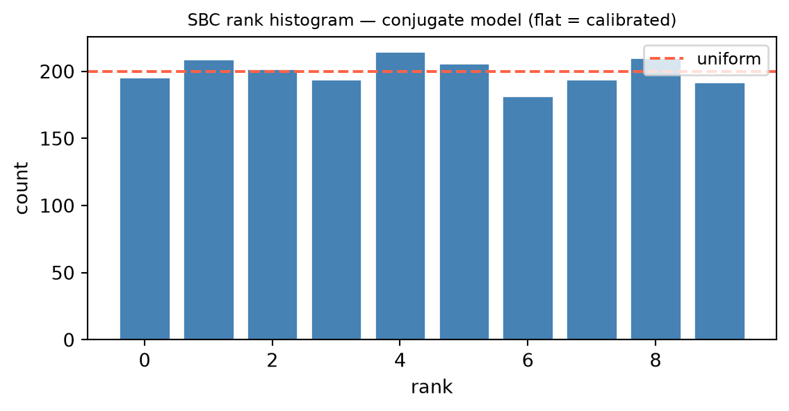
- Uniform (flat). The ranks are spread evenly across all bins: the inference is calibrated, exactly as the theorem demands.
- \cup-shaped (mass piled at both extremes). The truth lands in the tails of the posterior — at rank 0 or rank L — far too often. This is the signature of a posterior that is too narrow: an overconfident inference whose intervals are too tight and whose truth keeps falling outside them.
- \cap-shaped (mass bunched in the middle). The truth lands near the center of every posterior more often than chance allows. The posterior is too wide — an under-confident inference whose intervals are inflated.
- Sloped (ranks rising toward one end or falling toward the other). The posterior is biased: a histogram tilted toward high ranks means the posterior systematically sits below the truth (biased low), and a tilt toward low ranks means it sits above (biased high).
The shape diagnoses the disease, which is what makes SBC an instrument rather than a verdict.
Tie-back to Chapter 10: SBC catches the funnel
This is where the chapter’s threads converge. The funnel of Chapter 10 — the hierarchical geo model whose posterior pinches to a sliver as the group-scale \tau \to 0 — is a calibration failure waiting for an instrument that can see it, and SBC is that instrument, operating automatically. Fit the hierarchy in its centered parameterization, the one whose sampler cannot reach the funnel’s neck, and the posterior for \tau comes back biased and mis-dispersed because an entire region of the parameter space goes unvisited. Its \tau-rank histogram is then visibly non-uniform — sloped from the bias, \cup- or \cap-shaped from the mis-dispersion — and SBC fails the fit without anyone having to know in advance that a funnel was the culprit. Re-fit in the non-centered reparameterization, which flattens the funnel into a geometry the sampler can traverse, and the \tau-ranks fall flat: SBC passes. The qualitative funnel story of Chapter 10 — a pathology argued from pictures of trajectories getting stuck — becomes, through SBC, a quantitative and fully automatable test that fires on its own whenever the geometry defeats the sampler.
Rung 8 — Out-of-sample prediction: ELPD, WAIC, and LOO
Rungs 5 through 7 discharged B1: they asked whether a single fitted model is self-consistent — whether it reproduces its own training data and reports honest intervals. They are silent on a different question, the one a modeller actually faces when two specifications both pass their checks: which model predicts better? That is B2, and it is the business of model comparison, not model adequacy. A model can be perfectly self-consistent and still generalize worse than its rival; conversely, the better predictor is not always the one with the tighter posterior predictive overlay. The tools of this rung score predictive quality on data the model has not seen, and they are stated here precisely rather than proved — the asymptotic theory that justifies them is beyond this chapter, and the honest move is to cite it (Gelman et al. 2013; Vehtari et al. 2017) and use it correctly.
The target: ELPD. The quantity that scores predictive quality is the expected log pointwise predictive density for new data,
\text{elpd} = \sum_{i=1}^{n} \int p_t(\tilde{y}_i)\,\log p(\tilde{y}_i \mid y)\,d\tilde{y}_i,
where p_t is the true data-generating process and p(\tilde{y}_i \mid y) the model’s posterior predictive density. The log score is a proper scoring rule: it is maximized in expectation by the true predictive distribution, so it rewards calibration AND sharpness together — a model is scored well only when it concentrates probability on what actually happens, neither hedging with diffuse predictions nor committing confidently to the wrong values. ELPD cannot be computed: it requires both p_t, which we do not know, and new data, which we do not have. Everything that follows is machinery for estimating it from the fit in hand.
The naive estimate and why it overfits. The obvious surrogate evaluates the predictive density on the observed data themselves. This is the in-sample log pointwise predictive density,
\text{lppd} = \sum_{i=1}^{n} \log\!\left(\frac{1}{S}\sum_{s=1}^{S} p(y_i \mid \theta^{(s)})\right),
averaging the likelihood over S posterior draws \theta^{(s)}. Because it scores the model on exactly the data used to fit it, the lppd is optimistic — it credits the model for fitting noise it will not see again — and must be corrected downward by a penalty for the effective number of parameters the model spent.
WAIC. The widely applicable information criterion estimates ELPD by subtracting that complexity penalty directly,
\widehat{\text{elpd}}_{\text{WAIC}} = \text{lppd} - p_{\text{WAIC}}, \qquad
p_{\text{WAIC}} = \sum_{i=1}^{n}\operatorname{var}_{s}\!\bigl(\log p(y_i \mid \theta^{(s)})\bigr),
where the penalty is the posterior variance of the log-likelihood, summed over data points — an automatic count of the effective number of parameters that requires no fit beyond the posterior draws already in hand. A point whose log-likelihood swings widely across the posterior is one the model is flexibly bending to accommodate, and the variance charges for exactly that flexibility (Gelman et al. 2013; Vehtari et al. 2017).
PSIS-LOO. Leave-one-out cross-validation estimates ELPD more directly as \text{elpd}_{\text{LOO}} = \sum_i \log p(y_i \mid y_{-i}), the predictive density of each point under a fit to all the others. Done literally this demands n refits, one per held-out point — prohibitive for an MMM. Importance sampling avoids them: the leave-one-out predictive can be recovered from the single posterior already computed, reweighting its draws with importance weights proportional to 1/p(y_i \mid \theta^{(s)}). Those weights have heavy tails — a draw that fits point i poorly receives enormous weight — so they are stabilized by fitting a generalized Pareto distribution to the largest of them and replacing them with the fitted order statistics: Pareto-smoothed importance sampling (PSIS). The fitted Pareto shape parameter \hat{k}, computed per data point, is then a built-in reliability diagnostic. A value \hat{k} < 0.7 certifies that the importance-sampling estimate for that point is trustworthy; a value \hat{k} > 0.7 flags a point whose leave-one-out estimate is unreliable — typically a high-leverage observation whose removal would shift the posterior so much that the full-data draws are a poor proxy for the leave-one-out fit (Vehtari et al. 2017).
Equivalence and use. WAIC and PSIS-LOO are asymptotically equivalent: both are consistent estimators of the same ELPD, and in large samples they agree. PSIS-LOO is generally preferred in practice for its better finite-sample robustness and, decisively, for its per-point \hat{k} diagnostic, which tells you when not to trust it — a safeguard WAIC lacks. In MMM these tools answer which specification predicts better: a model with a competitor-spend control against one without it, or two adstock decay forms against each other. The comparison is made on the difference in ELPD together with its standard error, never on either model’s checks read in isolation — an ELPD difference smaller than a couple of its standard errors is not evidence that one model out-predicts the other. This is B2, and it complements rather than replaces the B1 checks: a model must be self-consistent to be worth comparing, and must out-predict its rivals to be worth choosing.
Rung 9 — A model-checking workflow
The rungs of this chapter are not a menu to graze from; they are an ordered pipeline, each step catching a distinct failure that the steps before it cannot. Assembled into a workflow for an MMM, they run as follows.
- Prior predictive check. Before any data touch the model, simulate from the prior and inspect the implied datasets. This catches absurd priors — sales that go negative, ROAS curves with impossible curvature — while they are still cheap to fix.
- Fit, then convergence diagnostics. Run the sampler, then certify it: split rank-normalized \hat{R} < 1.01 on every parameter, adequate bulk-ESS and tail-ESS, Monte Carlo standard errors small against the scale of each estimand, and zero divergences. This catches a sampler that has not actually characterized the posterior — the Part A failure that makes every downstream number meaningless.
- Posterior predictive checks. Replicate data from the fitted model and compare to what was observed. This catches structural misfit: a model that cannot reproduce seasonal sales peaks, or that smooths away the promotional spikes that drive the business.
- Simulation-based calibration. Validate the entire inference procedure against the uniform-rank signal. This catches miscalibration and implementation bugs that every preceding check can pass over — the overconfident interval, the funnel the sampler silently failed to explore.
- PSIS-LOO. With a single trustworthy model in hand, compare candidate specifications on out-of-sample prediction, choosing by ELPD difference and its standard error.
The consequence for the rest of the book is not optional. Only a model that clears steps 1 through 4 should feed the budget optimizer of Part IV. A red light on divergences, or a non-uniform SBC histogram, means the ROAS posterior is untrustworthy — and an optimizer fed an untrustworthy posterior does not fail safely. It seeks out and amplifies precisely the misspecified directions, allocating budget toward whatever channel the model’s error happened to flatter; the optimization machinery turns a quiet inferential bug into a confident, expensive recommendation. This is why checking is not a postscript to modeling. It is the gate between a fitted model and a decision, and the gate must hold. A checked, trustworthy posterior — one that has passed every rung of this chapter — is exactly the input the optimization of Part IV assumes it has been handed.
Worked Examples
The three diagnostics that carry the most arithmetic — \hat{R}, effective sample size, and the SBC rank — are each small enough to compute entirely by hand. Doing so once fixes what the formulas of Rungs 2, 3, and 7 actually measure.
Example 1 — Computing \hat{R} from four chains
Take M = 4 chains, each of length N = 4, of a scalar parameter \theta:
- Chain 1: 3,\ 4,\ 5,\ 4
- Chain 2: 4,\ 5,\ 6,\ 5
- Chain 3: 2,\ 3,\ 4,\ 3
- Chain 4: 5,\ 6,\ 7,\ 6
We compute \hat{R} from the definitions of Rung 2.
Chain means and grand mean. Averaging each chain,
\bar\theta_1 = 4, \qquad \bar\theta_2 = 5, \qquad \bar\theta_3 = 3, \qquad \bar\theta_4 = 6,
and the grand mean is \bar\theta = \frac{1}{4}(4 + 5 + 3 + 6) = 4.5.
Within-chain variances. Every chain has the shape \{m-1,\ m,\ m+1,\ m\} around its own mean m, so its deviations are \{-1,\ 0,\ +1,\ 0\} regardless of m. Each within-chain sample variance uses the denominator N - 1 = 3:
s_m^2 = \frac{(-1)^2 + 0^2 + (+1)^2 + 0^2}{3} = \frac{2}{3} \qquad \text{for every } m.
The within-chain estimate is their average,
W = \frac{1}{M}\sum_{m=1}^{M} s_m^2 = \frac{1}{4}\Bigl(4 \cdot \tfrac{2}{3}\Bigr) = \frac{2}{3} \approx 0.6667.
Between-chain variance. The squared deviations of the chain means from the grand mean are
\sum_{m=1}^{M}(\bar\theta_m - \bar\theta)^2 = (4 - 4.5)^2 + (5 - 4.5)^2 + (3 - 4.5)^2 + (6 - 4.5)^2 = 0.25 + 0.25 + 2.25 + 2.25 = 5,
so, with B = \frac{N}{M-1}\sum_m(\bar\theta_m - \bar\theta)^2,
B = \frac{4}{3} \cdot 5 = \frac{20}{3} \approx 6.6667.
Marginal variance estimate and \hat{R}. Combining the two with the weights of Rung 2,
\widehat{\operatorname{var}}^+(\theta) = \frac{N-1}{N}\,W + \frac{1}{N}\,B = \frac{3}{4}\cdot\frac{2}{3} + \frac{1}{4}\cdot\frac{20}{3} = \frac{1}{2} + \frac{5}{3} = \frac{13}{6} \approx 2.1667,
and therefore
\hat{R} = \sqrt{\frac{\widehat{\operatorname{var}}^+(\theta)}{W}} = \sqrt{\frac{13/6}{2/3}} = \sqrt{\frac{13}{4}} = \sqrt{3.25} \approx 1.8028.
Interpretation. The result \hat{R} \approx 1.80 \gg 1.01 fails the convergence threshold by a wide margin. The four chains sit in systematically different places — their means 3, 4, 5, 6 are spread far wider than the wobble within any one chain — so the between-chain term B dwarfs W and the ratio blows up. This is the textbook signature of an unmixed hierarchy whose between-group scale \tau is poorly identified: the geo-MMM funnel, with each chain trapped near a different value of the weakly constrained parameter.
Example 3 — A simulation-based calibration rank
In one SBC replication of the kind constructed in Rung 7, the ground truth drawn from the prior is \theta_0 = 0.7, and the inference under test returns L = 9 posterior draws, which sorted are
-0.2,\ 0.1,\ 0.3,\ 0.55,\ 0.8,\ 0.9,\ 1.1,\ 1.3,\ 1.6.
The rank. By the definition r = \#\{\ell : \theta_\ell < \theta_0\}, the rank counts how many posterior draws fall below \theta_0 = 0.7. The four draws -0.2, 0.1, 0.3, 0.55 are below 0.7; the five draws 0.8, 0.9, 1.1, 1.3, 1.6 are above. Hence
r = 4,
one of the L + 1 = 10 possible values 0, 1, \dots, 9 — ten bins in all.
Interpretation. One rank is almost uninformative: a single draw of a \text{Uniform}\{0, \dots, 9\} variable, by the theorem of Rung 7, tells us essentially nothing on its own. The diagnosis lives in the aggregate histogram over many replications, and its shape is what convicts or acquits the inference. Two contrasting cases make the point. A flat histogram, with the ranks spread evenly across all ten bins, is exactly the uniform signal the theorem demands — the inference is calibrated. A \cup-shaped histogram, with mass piled into bins 0 and 9, is the signature of an overconfident posterior: the truth keeps landing in the extreme bins because the posterior intervals are too narrow, so the ground truth falls into the tails — at rank 0 or rank L — far more often than chance allows. This is precisely the reading of histogram shapes set out in Rung 7, where the \cup shape diagnoses a posterior that is too narrow.